
Summary
- When constructing a coding solution to an implememtation problem, or an algorithm/theory for a mathematical problem, we can get bogged down in detail and lose our way.
- Abstraction helps us to move up a level and leave the detail behind.
- Once we temporarily leave the detail behind, what we need to do becomes clearer.
- Now we know what we have to do or implement, we can successfully put the detail back in because we have a clear ‘north star’ of what we need to implement.
Introduction
The computer scientist Edsger Dijkstra once said,
The purpose of abstracting is not to be vague, but to create a new semantic level in which one can be absolutely precise.
This is one of my favourite computing-related quotes, not least because it comes from Dijkstra. Edsger Dijkstra was a prodigious and extremely impactful computer scientist. In 1972 he was awarded the ACM A.M. Turing prize, widely regarded as the “Nobel prize for computer science”. Dijkstra was also “the computer scientist’s computer scientist”, providing rigorous solutions to tough practical problems, such as finding the shortest path between any two nodes on a network.
I also like the Dijkstra quote because I can relate to it. Whenever I want clarity on a problem, I abstract. Abstraction allows me to identify and focus on the “what” by taking the details of the “how” out of the discussion (for the time being). Once I know “what” it is I need to do I can put the details of the “how” back in and it becomes a straightforward technical implementation task (with debugging of course).
Yes, I hear you say, but what do you actually mean by all this high-level philosophical talk? I’ll give you two example. Yes, they are concocted examples, but they help illustrate what I’m driving at. Once I’ve discussed the two examples, we can then distil a more general approach of, i) when to recognize that we need more abstraction, and ii) how to do it.
Example 1:
Imagine you have the following equation,

In Eq.1 


I will now tell you that Eq.1 represents the field equations for Einstein’s theory of general relativity. With just high-schools maths you’ve been able to understand general relativity. 

All of the physics concepts of Einstein’s theory are in that simple equation of Eq.1 and likewise in the simple sentence from Wheeler. At this abstract level, the “what”, i.e. the physics, is crystal clear. However, when we start getting into the technical detail we have to go deeper. To “implement” a calculation we have to start to get to grips with the “how” and learn about Christoffel symbols, Ricci tensors, covariant and contravariant tensors, and much more. It requires mathematical training.
The details are also a lot messier. In the way I have presented the example, we started with the abstraction and then introduced some of the detail. When we are actually doing research, it is usually the reverse. We start with some existing details and want to construct a simplifying, unifying theory, but we get lost in the details because of the deep technical nature of those details.
A similar thing can happen when we are coding a Data Science solution. When we are deep in the technical details we often fail to spot the high-level patterns and so we fail to spot the simple description. We end-up producing lots of corner-cases and edge-cases. Our code starts to become one big series of “if-else if” statements or a big “switch” statement. Our second example illustrates that in a Data Science context.
Example 2:
In our first example we established that we are comfortable with linear models. In statistics a linear model is of the form,

The left-hand side of Eq.2 is the mean of our target variable 

What about non-linear models? Imagine that we have a non-linear relationship between our target variable and a single explanatory feature 
Let’s move away from the details about how we do the model fitting and focus on what we want. Let’s abstract. We want to model the mean of the target variable. When we state the problem in these simple terms we realise we can just write the mean of the target variable as a non-linear transformation of the linear predictor in Eq.2. We write this as,

This is what statisticians call a Generalized Linear Model (GLM). Again, the left-hand side of Eq.3 is how we represent the mean of the target variable 

The way we introduced Eq.3 seemed very natural and intuitive. And yet so many Data Scientists seem scared of GLMs. The jargon of link functions and the notation of expectation values 
What can we learn more generally from those two examples?
How to use abstraction as a practical tool
What the two examples above will hopefully have convinced you about is:
- Focusing at a high-level on the ‘things’ in our problem and what we want them to do helps us to identify the main actors in problem, the relationships between them and what we need to do to them. We discover the “what”.
- Once we have the what, the “how”, i.e. the implementation is typically easy.
But how to use this in practice? Whenever I find myself trying to solve a coding problem and I’m getting bogged down in the details of structuring the problem, flipping between different choices of data-structures to use, then I know I’m too close to the problem. I know I need to step away from the keyboard and get the pen and paper out.
I start by representing the main objects in my problem by some sort of symbol, e.g. a circle or a square. I then sketch out what interactions happen between those objects. By this point I’m beginning to describe the interactions in terms of high-level language such as, “I have matrix of type X. It is processed by a transform of type Y that is parameterized by mathematical object of type A”. You’ll spot that I’m already beginning to describe the interactions more in terms of interfaces and method signatures. That is, I’m focusing on the abstraction of the problem and not on the implementation details that would occur behind those interfaces and method signatures. This is because I have no other choice. I have only pen and paper. I can’t code, so I can’t bogged down again in implementation details and discussions on what data structures to use.
Once I have finished a couple of iterations of pen-and-paper sketching I have the architecture of my solution nailed. And the best thing is the structure typically mimics the structure of the actual mathematical calculation I’m trying to code. At this point I have identified what interfaces, classes, and methods I need. I now return to the keyboard and the implementation is easy.
Conclusion
If you’re getting bogged down in working out implementation details, it is a good sign you don’t actually know “what” it is you need to implement.
Step back, move up a level of abstraction and start identifying what are the things/actors in your problem and what are the interactions between them. Doing this using pen-and-paper will aid you a lot, because it forces you away from the keyboard and the temptation to continue implementing.
Once you have sketched out the necessary objects and their interactions you will pretty much have the classes, interfaces, and methods you need. You have the “what”. Now you can implement. It will now be a lot faster.
© 2026 David Hoyle. All Rights Reserved
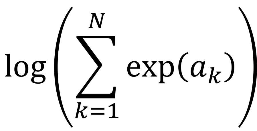
 . This calculation is called log-sum-exp.
 function.
 , where you have values for the
  . Really? Will you? Yes, it will probably be calculating a log-likelihood, or a contribution to a log-likelihood, so the actual calculation you want to do is of the form,
 and
and  and
and  to
to  we are using floating point arithmetic to try and add a very large number to a much smaller number. Most likely we will get an overflow error. If would be much better if we’d started with
  , which would be very negative and from this we could easily infer that adding
  by
by  and computes an accurate approximation to
  without encountering underflow or overflow errors.
![a = [a_{1}, a_{2}, \ldots, a_{N}]](https://s0.wp.com/latex.php?latex=a+%3D+%5Ba_%7B1%7D%2C+a_%7B2%7D%2C+%5Cldots%2C+a_%7BN%7D%5D&bg=ffffff&fg=111111&s=0&c=20201002) . Let’s say, without loss of generality, the maximum value is
. Let’s say, without loss of generality, the maximum value is 
 are all negative for
  , so we can easily approximate the logarithm on the right-hand side of the equation by a suitable expansion of
  . This is the “log-sum-exp” trick.

 , it is also relatively easy to show that,

 are allowed to be negative. This means, that when we are using the SciPy log-sum-exp function to perform the log-sum-exp trick, we can actually use it to calculate numerically stable estimates of sums of the form,
 .
. . This is because the first two contributions,
  .
.