How many iterations are needed for the bisection algorithm?

<TL;DR>

The bisection algorithm is a very simple algorithm for finding the root of a 1-D function.
Working out the number of iterations of the algorithm required to determine the root location within a specified tolerance can be determined from a very simple little hack, which I explain here.
Things get more interesting when we consider variants of the bisection algorithm, where we cut an interval into unequal portions.

</TL;DR>

A little while ago a colleague mentioned that they were repeatedly using an off-the-shelf bisection algorithm to find the root of a function. The algorithm required the user to specify the number of iterations to run the bisection for. Since my colleague was running the algorithm repeatedly they wanted to set the number of iterations efficiently and also to achieve a guaranteed level of accuracy, but they didn’t know how to do this.

I mentioned that it was very simple to do this and it was a couple of lines of arithmetic in a little hack that I’d used many times. Then I realised that the hack was obvious and known to me because I was old – I’d been doing this sort of thing for years. My colleague hadn’t. So I thought the hack would be a good subject for a short blog post.

The idea behind a bisection algorithm is simple and illustrated in Figure 1 below.

How the bisection algorithm works — Figure 1: Schematic of how the bisection algorithm works

At each iteration we determine whether the root is to the right of the current mid-point, in the right-hand interval, or to the left of the current mid-point, in the left-hand interval. In either case, the range within which we locate the root halves. We have gone from knowing it was in the interval $[x_{lower}, x_{upper}]$ , which has width $x_{upper}-x_{lower}$ , to knowing it is in an interval of width $\frac{1}{2}(x_{upper}-x_{lower})$ . So with every iteration we reduce our uncertainty of where the root is located by half. After $N$ iterations we have reduced our initial uncertainty by $(1/2)^{N}$ . Given our initial uncertainty is determined by the initial bracketing of the root, i.e. an interval of width $(x_{upper}^{(initial)}-x_{lower}^{(initial)})$ , we can now work out that after $N$ iterations we have narrowed down the root to an interval of width ${\rm initial\;width} \times \left ( \frac{1}{2}\right ) ^{N}$ . Now if we want to locate the root to within a tolerance ${\rm tol}$ , we just have to keep iterating until the uncertainty reaches ${\rm tol}$ . That is, we run for $N$ iterations where $N$ satisfies,

$\displaystyle N\;=\; -\frac{\ln({\rm initial\;width/tol})}{\ln\left (\frac{1}{2} \right )}$

Strictly speaking we need to run for $\lceil N \rceil$ iterations. Usually I will add on a few extra iterations, e.g. 3 to 5, as an engineering safety factor.

As a means of easily and quickly determining the number of iterations to run a bisection algorithm the calculation above is simple, easy to understand and a great little hack to remember.

Is bisection optimal?

The bisection algorithm works by dividing into two our current estimate of the interval in which the root lies. Dividing the interval in two is efficient. It is like we are playing the childhood game “Guess Who”, where we ask questions about the characters’ features in order to eliminate them.

Asking about a feature that approximately half the remaining characters possess is the most efficient – it has a reasonable probability of applying to the target character and eliminates half of the remaining characters. If we have single question, with a binary outcome and a probability $p$ of one of those outcomes, then the question that has $p = \frac{1}{2}$ maximizes the expected information (the entropy), $p\ln (p)\;+\; (1-p)\ln(1-p)$ .

Dividing the interval unequally

When we first played “Guess Who” as kids we learnt that asking questions with a much lower probability $p$ of being correct didn’t win the game. Is the same true for our root finding algorithm? If instead we divide each interval into unequal portions is the root finding less efficient than when we bisect the interval?

Let’s repeat the derivation but with a different cut-point e.g. 25% along the current interval bracketing the root. In general we can test whether the root is to the left of right of a point that is a proportion $\phi$ along the current interval, meaning the cut-point is $x_{lower} + \phi (x_{upper}-x_{lower})$ . At each iteration we don’t know in advance which side of the cut-point the root lies until we test for it, so in trying to determine in advance the number of iterations we need to run, we have to assume the worst case scenario and assume that the root is still in the larger of the two intervals. The reduction in uncertainty is then, ${\rm max}\{\phi, 1-\phi\}$ . Repeating the derivation we find that we have to run at least,

$\displaystyle N_{Worst\;Case}\;=\;\ -\frac{\ln({\rm initial\;width/tol})}{\ln\left ({\rm max}\{\phi, 1 - \phi \right \})}$

iterations to be guaranteed that we have located the root to within $tol$ .

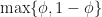
Now to determine the cut-point $\phi$ that minimizes the upper bound on number of iterations required, we simply differentiate the expression above with respect to $\phi$ . Doing so we find,

$\displaystyle \frac{\partial N_{Worst\;Case}}{\partial \phi} \;=\; -\frac{\ln({\rm initial\;width/tol})}{ (1-\phi) \left ( \ln (1 - \phi) \right )^{2}} \;\;,\;\; \phi < \frac{1}{2}$

and

$\displaystyle \frac{\partial N_{Worst\;Case}}{\partial \phi} \;=\; \frac{\ln({\rm initial\;width/tol})}{\phi \left ( \ln (\phi) \right)^{2}} \;\;,\;\; \phi > \frac{1}{2}$

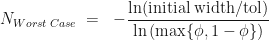
The minimum of $N_{Worst\;Case}$ is at $\phi =\frac{1}{2}$ , although $\phi=\frac{1}{2}$ is not a stationary point of the upper bound $N_{Worst\;Case}$ , as $N_{Worst\;Case}$ has a discontinuous gradient there.

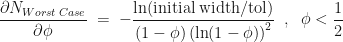
That is the behaviour of the worst-case scenario. A similar analysis can be applied to the best-case scenario – we simply replace $max$ with $min$ in all the above formula. That is, in the best-case scenario the number of iterations required is given by,

$\displaystyle N_{Best\;Case}\;=\;-\frac{\ln({\rm initial\;width/tol})}{\ln\left ({\rm min}\{\phi, 1 - \phi \right \})}$

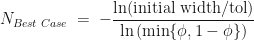
Here, the maximum of the best-case number of iterations occurs when $\phi = \frac{1}{2}$ .

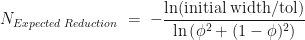
That’s the worst-case and best-case scenarios, but how many iterations do we expect to use on average? Let’s look at the expected reduction in uncertainty in the root location after $N$ iterations. In a single iteration a root that is randomly located within our interval will lie, with probability $\phi$ , in segement to the left of our cut-point and leads to a reduction in the uncertainty by a factor of $\phi$ . Similarly, we get a reduction in uncertainty of $1-\phi$ with probability $1-\phi$ if our randomly located root is to the right of the cut-point. So after $N$ iterations the expected reduction in uncertainty is,

$\displaystyle {\rm Expected\;reduction}\;=\;\left ( \phi^{2}\;+\;(1-\phi)^{2}\right )^{N}$

Using this as an approximation to determine the typical number of iterations, we get,

$\displaystyle N_{Expected\;Reduction}\;=\;-\frac{\ln({\rm initial\;width/tol})}{\ln\left ( \phi^{2} + (1-\phi)^{2} \right )}$

This still isn’t the expected number of iterations, but to see how it compares Figure 2 belows shows simulation estimates of $\mathbb{E}\left ( N \right )$ plotted against $\phi$ when the root is random and uniformly distributed within the original interval.

The number of iterations needed for the bisection algorithm — Number of iterations required for the different root finding methods.

For Figure 2 we have set $w = ({\rm initial\;width/tol}) = 0.01$ . Also plotted in Figure 2 are our three theoretical estimates, $\lceil N_{Worst\;Case}\rceil, \lceil N_{Best\;Case}\rceil, \lceil N_{Expected\;Reduction}\rceil$ . The stepped structure in these 3 integer quantities is clearly apparent, as is how many more iterations are required under the worst case method when $\phi \neq \frac{1}{2}$ .

The expected number of iterations required, $\mathbb{E}( N )$ , actually shows a rich structure that isn’t clear unless you zoom in. Some aspects of that structure were unexpected, but requires some more involved mathematics to understand. I may save that for a follow-up post at a later date.

Hoyle Analytics

How many iterations are needed for the bisection algorithm?

<TL;DR>

</TL;DR>

Is bisection optimal?

Dividing the interval unequally

Leave a Reply Cancel reply

<TL;DR>

</TL;DR>

Is bisection optimal?

Dividing the interval unequally

Share this:

Like this:

Leave a Reply Cancel reply