Data Science Notes: 5. Trimmed variances and getting MAD

On May 29, 2026May 29, 2026 By dchoyleIn Data Science, Data Science Notes, StatisticsLeave a comment

Summary

Estimating the variance of a distribution when we have outliers can create a circular problem, particularly if we want to use the estimated variance in an algorithm to detect the outliers in the first place.
If we are prepared to assume, that at most, a fraction $\alpha$ of our data are outliers, then we can use a trimmed-variance to estimate the population variance without having to explicitly identify the outliers.
We incorporate a correction factor to make our variance estimate consistent with the parametric distribution we have assumed our data has been drawn from.
The median absolute deviation from the median (MAD) also uses a similar idea and tends to have better performance (efficiency) for outlier-contaminated Normal data.
Calculating the Normal-consistent MAD-based estimate of the standard deviation is ridiculously simple.

Introduction

This is one of those little hacks that I really like. So simple, so easy, and yet it solves a real problem. It solves a circular problem. How to estimate the standard deviation of a distribution from a sample of data, without being impacted by outliers when we haven’t yet identified which datapoints are outliers. We may even want to use that estimate of the standard deviation to help detect those outliers – in an appropriate algorithm that takes the sample size into account of course (see my previous Data Science Notes post What is an outlier?). It looks like we have a circular problem; the outliers affect the estimation of the standard deviation, but we can’t identify and deal with those outliers until we have calculated the standard deviation.

We can drop the data points from the tails of the sample to remove outliers. The trouble is the standard deviation relates to the spread of values in a distribution, i.e. it relates to the tails of the distribution. It looks like we are going to lose signal about the standard deviation if we do this.

If only there was a way to estimate a standard deviation from just the data values around the mean. That is, can we estimate the standard deviation from the data points that have come from the bulk of the distribution and not its tails? There is, if we are prepared to make a parametric assumption about the shape of the distribution. Once we make a parametric assumption about the shape, any datapoint gives us signal about the parameters of the distribution. And once we have signal about the parameters of the distribution we have signal about its standard deviation.

Theory

Let’s use the Normal distribution as an example. We know that the probability density is given by,

$\phi (x)\;=\; \frac{1}{\sqrt{2\pi\sigma^{2}}}\exp \left ( -\frac{1}{2\sigma^{2}}\left ( x - \mu\right )^{2}\right )$ Eq.1

In Eq.1 $\mu$ is the mean of the probability distribution and $\sigma$ is its standard deviation. The part of the probability distribution that corresponds to the central 90% of the probability distribution is given by the interval $\left [ -\sigma x_{5} + \mu , \sigma x_{5} + \mu \right ]$ , where $x_{5}$ corresponds to the 5^th centile of the standard Normal distribution and so is given by,

$x_{5} \;=\; -\sqrt{2} {\rm erf}^{-1}\left ( 0.95 \right )$ Eq.2

If we calculate the 2^nd moment of $x$ about the mean $\mu$ and over that central 90% portion of the probability distribution we can write that,

$\frac{1}{\sqrt{2\pi\sigma^{2}}}\int_{-x_{5} }^{x_{5}} x^{2}\,\exp \left ( -\frac{x^{2}}{2\sigma^{2}}\right )\, dx\;=\; 0.9\sigma^{2}\left [ 1 + \frac{2}{0.9}\Phi^{-1}\left ( 0.05\right ) \phi \left ( \Phi^{-1}\left ( 0.05 \right )\right ) \right ]$ Eq. 3

In Eq.3 $\Phi(z)$ is the CDF of the Standard Normal distribution and so $\Phi(z) = \frac{1}{2}{\rm erfc}\left ( -z/\sqrt{2} \right )$ . The right-hand side of Eq.3 is 0.9 times what we would get if we had an infinite sample of data from a Normal distribution with standard deviation of $\sigma$ and removed the upper and lower 5% of the datapoints and then calculated the sample standard deviation $s^{2}$ .

Let’s denote our sample of data by the vector $\underline{x}$ . Eq.3 tell us that once we have removed the upper and lower 5% of datapoints from our sample $\underline{x}$ and then calculated $s^{2}$ , we have,

$s^{2} \simeq \sigma^{2}\left [ 1 + \frac{2}{0.9}\Phi^{-1}\left ( 0.05\right ) \phi \left ( \Phi^{-1}\left ( 0.05 \right )\right ) \right ]$ Eq.4

A simple re-arrangement of Eq.4 gives us a means of estimating $\sigma^{2}$ from our trimmed data sample. We just use,

$\hat{\sigma}^{2}\simeq \frac{s^{2}}{\left [ 1 + \frac{2}{0.9}\Phi^{-1}\left ( 0.05\right ) \phi \left ( \Phi^{-1}\left ( 0.05 \right )\right ) \right ] }$ Eq.5

There you have it. A simple way to estimate the standard deviation of a Normal distribution whilst excluding the smallest and largest 5% of values. If we want to exclude $\alpha \times 100\%$ of values, we can easily generalize the formula in Eq.5. I’ll leave it to you as an exercise to do the derivation. I’m just going to quote the final result below,

$\hat{\sigma}^{2}\;=\; \frac{s^{2}}{\left [ 1 + \frac{2}{1 - \alpha}\Phi^{-1}\left ( \frac{1}{2}\alpha\right ) \phi \left ( \Phi^{-1}\left ( \frac{1}{2}\alpha \right )\right ) \right ] }$ Eq.6

Practice

That’s the theory. How do we use this simple idea in practice? Like all simple but great ideas someone has already coded it up for you. In Python the trimmed variance of an array a of numbers can be calculated using the trimmed_var function in scipy.stats.mstats, as follows,

			
from scipy.stats.mstats import trimmed_var
trimmed_var = trimmed_var(a,
                          limits=(0.05, 0.05),
                          inclusive=(1, 1),
                          relative=True,
                          axis=None,
                          ddof=1)

		

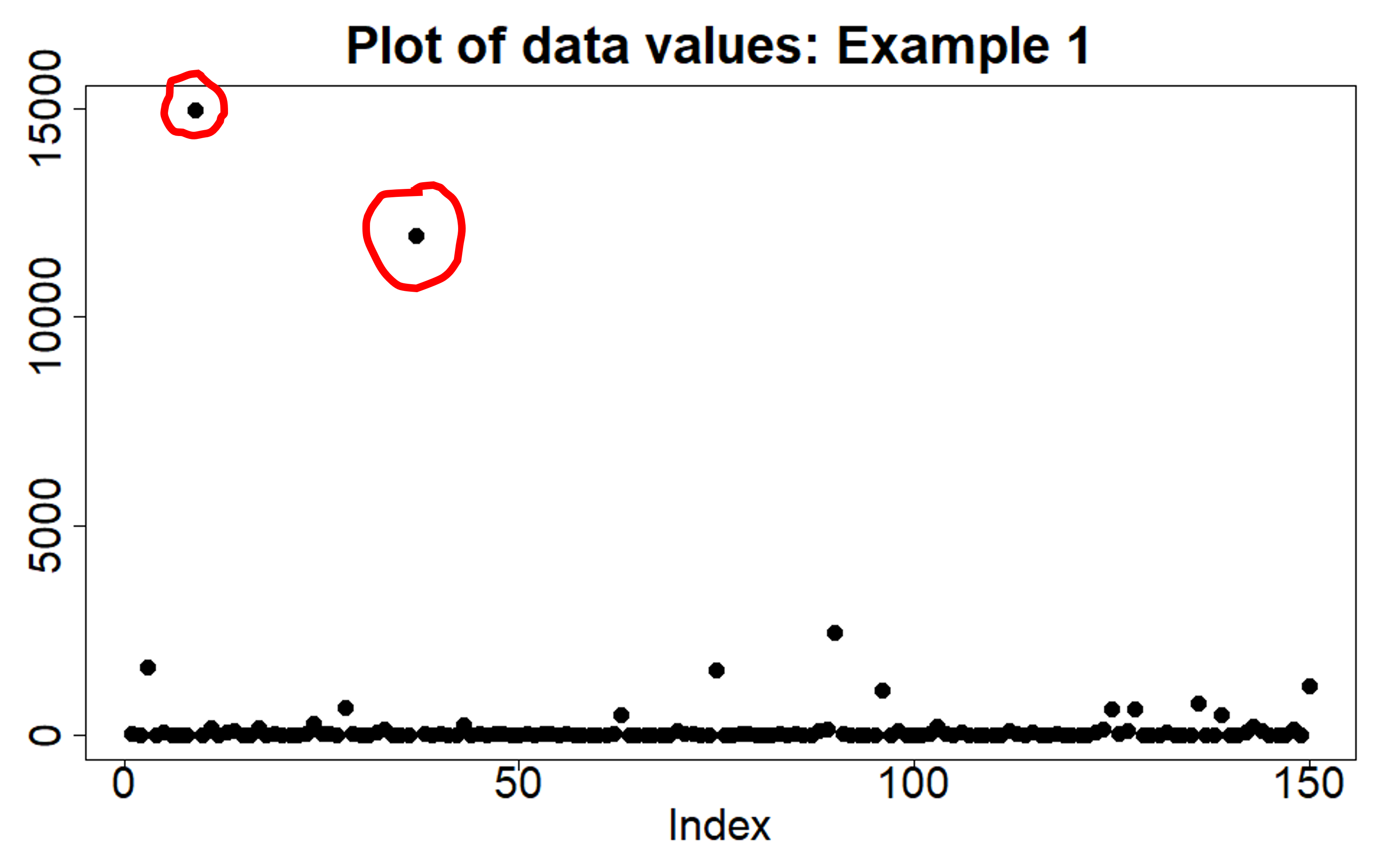
In the notebook DataScienceNotes5_TrimmedVariances.ipynb in the public GitHub repository github.com/dchoyle/datascience_notes, I have used the trimmed_var function to run a number of simulations. The plot below (Figure 1) shows the average estimated variance, averaged over 1000 simulation datasets, using the formula in Eq.6 and where I have used the scipy trimmed_var function to calculate $s^{2}$ for each simulation sample. The plot shows the average (over simulation datasets) estimated population variance at a number of different sample sizes $N$ and for three different values of $\alpha$ .

Figure 1: Plot of the simulation means for the trimmed-variance estimates against log N.

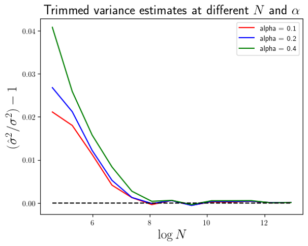
On the y-axis I’ve actually plotted the ratio of the average estimated variance to the true population variance (with which the data was generated) minus 1, so that it is easier to see how accurate the estimated variance is. A value of zero on the y-axis indicates a perfect estimate. You can see that as the starting sample size $N$ increases, each of the different $\alpha$ curves converges to zero, i.e. a perfect estimate, on average, of the true variance. However, the rate of convergence appears to be diffferent for the different values of $\alpha$ . In part, this is illusory, and is because we haven’t adjusted the x-axis for the effective sample size. Conisder if our starting sample size was $N=10000$ . At $\alpha=0.1$ we are actually estimating the variance from 900 data points. The effective sample size is 900. Whilst for $\alpha=0.4$ the variance is estimated from a trimmed sample consisting of 600 data points. In order to compare like effective sample sizes with like effectve sample sizes I simply need to adjust the x-axis values in Fig.1 by $\log(1-\alpha)$ . This I have done in Figure 2 below.

Figure 2: Plot of the simulation means of the trimmed-variance estimates plotted against the adjusted sample size.

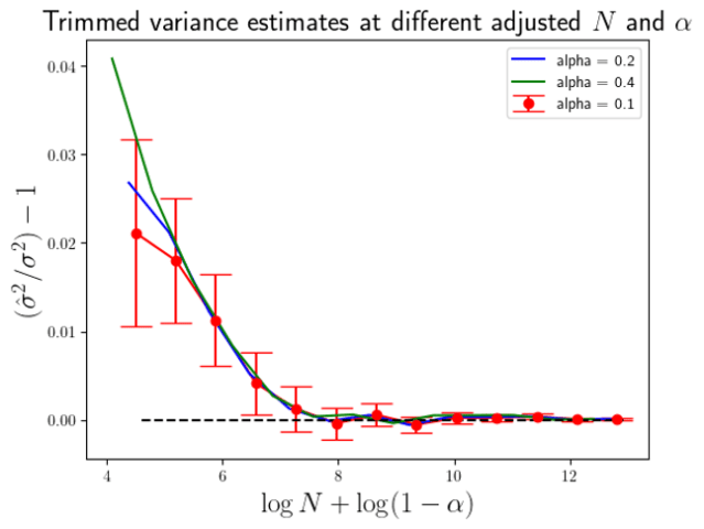
You can see that in Fig.2 all three different $\alpha$ curves are nearly identical, particularly at the larger values of $N$ . In Fig.2 I have also included error bars on the $\alpha=0.1$ curve. These correspond to $\pm 2$ times the standard errors of the means in the $\alpha=0.1$ curve. I haven’t included the standard errors for the other two curves simply because they will be of similar scale and will make the plot too crowded. From Fig.2, with the standard errors visible we see that there is a bias in the variance estimates at smaller values of $N$ , i.e. the average estimate is systematically different from the true population level. Deriving the mathematical form of the bias is a lengthy and challenging mathematical calculation, so I’m not going to go into it here.

Getting MAD

So far we have been calculating trimmed variances. However, the idea of using the central portion of a data sample to estimate a population quantity is more widely applicable. One of my favourite and most well known applications of this idea is the median absolute deviation, or MAD for short.

MAD is the median absolute deviation of $x$ from some measure of central tendency of $x$ , such as the median or mean. Usually, the default is to use the median as the measure of central tendency, so that the MAD is calculated as the median absolute deviation from the median. That is, we take our sample of data, calculate its median, calculate the absolute difference between each data point and that median, and calculate the median of all those absolute values.

The great thing about MAD (when using the median central tendency measure) is that for a large sample of data drawn from a Normal distribution, there is a very simple relationship between the expectation value of MAD and the population standard deviation $\sigma$ . That relationship is,

$\mathbb{E}\left ( {\rm MAD} \right ) \;\rightarrow\; \sigma \Phi \left ( 3/4 \right )\;=\; 0.6745\sigma\;\;\;,\;\; {\rm as} \;N\rightarrow\infty$ Eq.7

Let’s unpack what Eq.7 is telling us. It says that, on average, the MAD calculated from a sample of (Normally distributed) data is a simple constant times the true standard deviation. This means we can invert Eq. 7 to get a extremely simple way of estimating the population standard deviation that is robust to the presence of outliers (provided they make up less than 50% of the sample). That simple way is,

$\hat{\sigma}\;=\; 1.4826 \times {\rm MAD} \left ( \underline{x} \right )$ Eq. 8

Calculating the MAD is such a common task that once again you will find that most programming languages used for numerical analysis will contain a MAD function either as part of the base distribution, or in a commonly used package. In R we can use the mad function which is part of the base R distribution. In Python we can use scipy.stats.median_abs_deviation. In both cases the use of MAD to estimate the standard deviation is such a common use of MAD that both the R and Python functions have the correction factor of 1.4826 built in. In R, it is included by default, meaning that if you call mad, it will return the Normal adjusted estimate of $\sigma$ (also called the Normal consistent estimate). Be aware of this in case what you actually wanted was just the MAD value for a sample of data, rather than the Normal consistent estimate of $\sigma$ calculated from MAD. In Python, for the scipy.stats.median_abs_deviation function we have to explicitly tell it that we want the correction factor applied. We do that by setting the scale argument of the function equal to ‘normal’. The code-snippet below illustrates the scipy.stats.median_abs_deviation function in action.

			
from scipy.stats import median_abs_deviation
mad_sd_estimate = median_abs_deviation(a, scale='normal')

For the simulated data used to produce Fig.1 and Fig.2, I also calculated the MAD based estimate of $\sigma$ . The plot below (Figure 3) shows the simulation average of the Normal consistent MAD-based estimates of the true standard deviation $\sigma$ . The simulation averages are plotted against $\log N$ . Again, I have actually plottted the ratio of the simulation average of $\hat{\sigma}$ to $\sigma$ then minus 1. The dashed line is at a value of zero on the y-axis and is used to indicate when we have a bias in our estimate. The points are the means of the simulation results, i.e. the mean of the estimates of $\sigma$ over all the simulation datasets for the particular value of $N$ . The error bars correspond to $\pm$ 2 standard errors of the simulation means, with the standard error simply estimated from the variance over the simulation results.

Figure 3: Plot of the simulation means of the MAD-based estimates of the standard deviation, plotted against log N.

From Fig.3 we can see that the accuarcy of the MAD-based estimate of $\sigma$ is very good. This would appear (from the plot) to be a consistent estimator. Again we can see evidence of the bias in the estimator at the smaller values of $N$ . However, we can’t yet do a comparison with the trimmed-variance estimator, as we are estimating a different quantity. The trimmed-variance estimates the underlying population variance, whilst the MAD-based estimator estimates the underlying population standard deviation. Fortunately, when I computed the MAD-based estimates, I also stored the effective estimates of the variance, so we can do a like-for-like comparison with the trimmed-variance estimator. The MAD-based estimates of $\sigma^{2}$ are shown in the plot in Figure 4 below.

Figure 4: Plot of Normal-consistent MAD-based estimates of the population variance plotted against log N.

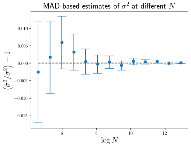
The accuarcy of the MAD-based estimator appears to be, at least for these simulation results, superior to the trimmed-variance estimator, with the errors being around $\pm$ 1%. The number of simulation runs is not sufficient in this set of results to properly detect the bias even for the smallest values of $N$ . However, given the plot in Fig.3, we would expect that if we increased the number of simulation runs appropriately, we would be able to resolve this, i.e. it is simply that the standard errors of the mean of $\hat{\sigma}^{2}/\sigma^{2}$ are larger than the standard errors of the mean of $\hat{\sigma}/\sigma$ (for this MAD-based estimator).

Other distributions

So far we have been discussing outlier-contaminated Normal data. But what happens if we are certain our data wasn’t drawn from a Normal distribution with an additional outlier process on top? What happens if we think our data is Gamma-distributed with outliers? We can still apply the same ideas, but it can get trickier and also more computationally intensive. Specifically, we need to distinguish two cases:

The distribution we assume is still symmetric about its mean – in this case calculating the trimmed variance with an appropriate correction factor, or calculating MAD with an appropriate correction factor is still relatively straight forward. The correction factors may not be expressable in terms of common special functions, or in the worst case you may have to evaluate them numerically, once you have reduced the calculation down to some canonical form.
The assumed distribution is not symmetric about its mean – in these circumstances it can become a lot trickier. Obviously, now things such as the skewness of the distribution affect the value of MAD or the trimmed-variance value, and so calculation of the correction factors is now affected by the shape of the distribution. This means we typically need to estimate a ‘shape’ parameter of the parametric distribution as well as estimating the ‘scale’ parameter of the distribution, which is the thing we are predominantly interested in. This will mean solving for shape and scale parameters simultaneously, and we are probably going to have to do that root finding numerically, as it is unlikely we can do it analytically. Calculating the appropriate adjustment factors is usually possible in these circumstances, but is typically more computationally intensive and/or we have to introduce additional approximations.

Conclusions

In many situations we want to estimate the standard deviation of a distribution from a sample of data, but we know there are outliers present in the sample.
We can’t use our usual estimate of the standard deviation to detect the outliers, because that estimate is affected by the outliers.
By making an assumption about the parametric form of the distribution whose standard deviation we are trying to estimate, we can estimate the standard deviation using data from any part of the distribution. This means we can use just the middle part of the sample data.
If we throw away a fraction $\alpha$ of the data, we can easily compute the correction factor needed, based upon our parametric assumption of the distribution shape.
In R and Python there are convenient functions for calculating the trimmed-variance of a sample and also the Normal-consistent MAD-based estimate of the population standard deviation.
Calculation of trimmed-variance and MAD-based estimates of variance is possible for distributions other than the Normal but will be more computationally intensive, particularly for asymmetric distributions.

Data Science Notes: 4. What is an outlier?

On March 9, 2026March 9, 2026 By dchoyleIn Data Science, Data Science Notes, Statistics1 Comment

Summary

What defines an outlier is something that causes a great deal of confusion amongst Data Scientists. Most Data Scientists get this wrong.
An outlier is not just simply a datapoint that has a very large or very small value.
My personal definition of an outlier is, “a datapoint that comes from a different statistical process than the one I’m currently modelling”.
Since real world data is typically made from multiple statistical processes, it is better to think not in terms of a dataset being comprised of “ok data + outliers”, but instead to think of data as being comprised from data from process 1, plus data from process 2, and so on.
Throwing away outliers is not a good idea. They made up part of your real dataset so you are throwing away insight into how your data gets generated. It is ok however to exclude “outliers” from estimation of the parameters of a specific statistical process if you have confidently identified those “outliers” as coming from a different mechanism.

Introduction

The image above is a well known meme, right. It’s quite funny, right? Yes, except I have seen this precise situation happen. 25 years ago I went to a talk where a scientist was presenting some experimental gene expression work they’d been doing. As they were using a new assay technology called ‘microarrays’, which they were concerned could provide noisy measurements, they’d decided under advice from another scientist to throw away any datapoints that were more than +/- 2 standard deviations from the mean of their data. My colleague and I, who were working on the theory of statistical analysis of microarray data, asked how much data they’d discarded. “It’s quite weird. We always seem to end up removing about 5% of the total data, no matter what experiment we do” was the reply. I’ve remembered that reply word for word since then.

What do you think an outlier is?

Take a look at the plot below. It is a dataset of 150 datapoints, with the values plotted on the y-axis and the index of each datapoint on the x-axis. Which datapoints do you think might be outliers? Possibly the ones I’ve circled in red, as they are clearly much larger than the bulk of the data points. Perhaps we should discard them?

Plot of example data points with two data points circled in red as possible outliers — An example dataset with possible outliers highlighted in red.

Okay, what about this second plot below? Again, a dataset of 150 datapoints. Probably no outliers right? All the data points are reasonably clustered together on the y-axis. Yes, some are more towards the edges but you would think you could easily model the distribution of this data using a single Gaussian distribution.

An example dataset with no outliers highlighted — A second example dataset

The two plots are of the same data.

How is this so? The data is drawn (simulated) from a log-normal distribution. The second plot shows the data values on a log scale, and as we’ve already commented we would be happy modelling the distribution of the data using a Gaussian distribution, using all the data points to estimate the mean and variance of that Gaussian distribution. The first plot shows the data on the original scale – sometimes we refer to this as the ‘normal scale’, but not to be confused with ‘normal’ as in ‘normal distribution’, we just mean we haven’t taken the logarithm. And yet, now we know that the appropriate distribution to use to model this data is a log-normal distribution, we are happy to use all the datapoints in the first plot to estimate the parameters of that log-normal distribution. There is no need to discard or throw away any datapoints.

What have we learnt from this little experiment? Two things:

Whether a datapoint is an outlier or not has nothing to do with how big the data value is.
If a datapoint is consistent with the statistical distribution or process we are trying to model, then we can use it. It is not an outlier, no matter how big or small it is.

The second point is my favourite way of defining an outlier. An outlier is a datapoint that comes from a statistical process other than that process which we are currently trying to model. Okay, that definition sounds a bit dry and technical, but I like it because it emphasizes that an outlier is not ‘wrong’, ‘incorrect’ or ‘deficient’ in any sense. It has not ‘corrupted’ or ‘contaminated’ the dataset in any true sense, even though those are common terms used in statistics when discussing robust parameter estimation methods. Instead, saying that a datapoint is an outlier just means we are saying it comes from a different mechanism than the one we are currently modelling. All the datapoints in the two plots above came from the same statistical process. I know because that is how I generated them.

The definition of an outlier I have just given also tells us why we are justified in omitting (not throwing away) outliers when estimating the parameters associated with the statistical mechanism we want to model. If a datapoint hasn’t come from the statistical mechanism we want to model, including it in any estimation or training algorithm will lead to incorrect parameter estimates. So once we are confident we have correctly identified any outliers, omitting them from the parameter estimation process is justified.

An illustration

Let’s we want to estimate the typical energy usage per square metre of rooms in a residential house. I can get data on a load of houses; the total energy use, the number of rooms, and the total floor aera of those rooms. It’s an easy calculation to then work out the average energy consumption per square metre. But if I notice that several of the ‘houses’ in my dataset have over 150 rooms each, I‘m probably going to think that they are not typical residential houses. Most likely they are hotels, or mansions of some tech billionaires. Either way, the pattern of energy usage for the rooms in those hotels/mansions is likely to be very different from that of a room in a typical residential house. The energy usage for those hotel rooms comes from a different statistical process to that for the residential house rooms. The datapoints from those hotels are outliers to what I’m trying to model. I should therefore exclude them from my estimation algorithm. That’s easy to do now that I’m am confident I have identified the outliers appropriately. Job done!

Life (and data) is always made up of multiple processes

The other reason I like the outlier definition I have given is that it emphasizes that real data is almost always made up of data coming from multiple mechanisms or processes. The outlier definition I’ve used highlights that an outlier isn’t wrong, it’s just different. Sometimes we only want to model in depth just one of the statistical mechanisms contributing to our dataset, so we omit the outliers and run our training algorithm. Other times we need to model all of the data in our dataset and so we break down our dataset into the different generative processes/mechanisms that we think are at play, select the appropriate subset of data for each process, and run an appropriate training algorithm on that subset. Instead of thinking of the data as being made up of ‘good’ data plus ‘outliers’, I now think of it as, ‘data from mechanism 1’ plus ‘data from mechanism 2’ plus ‘data from mechanism 3’, and so on.

Let’s revisit our energy consumption example to illustrate this. Say, now I want to model energy use per square metre for different types of buildings – residential houses and hotels. Now it is just a question of filtering the data to the datapoints matching the building type. As we said before, the energy use patterns will probably be different for houses and for hotels, i.e. we have different statistical processes generating the different subtypes of data. Consequently, we choose to use different distribution types to model the different building types. So what we have is not outliers, just a different training process for each of the different building types.

How to detect outliers?

So far I have only discussed how to think about what an outlier is. I’ve said that you are justified in excluding genuine outliers from parameter estimation once you have correctly identified them. What I have not discussed is how you actually do the outlier detection. That is deliberate, as it is a much bigger topic. It is also one I will touch upon, in part, in later posts in the Data Science Notes series.

What you will hopefully have grasped is that if we are to use something like standard deviation (SD) to determine whether a datapoint is an outlier, we need to replace the naive “|x – mean | > 2SD” filter shown in the meme image at the start and replace it with a question that asks whether the datapoint is consistent with a statistical process that has the given mean and SD. So we need to replace the meme with a question more like, “what is the probability of the highest value in a dataset of size N being greater than x?” We can see that outlier detection now takes into account the sample size and brings us into the realm of extreme value theory (EVT) – also a topic for a later Data Science Note.

Conclusions

An outlier is a datapoint that has come from a statistical process different to the one we are currently modelling.
Excluding outliers from parameter estimation for the statistical process we are currently modelling is valid because they don’t, by definition, conform to that statistical process and so would bias the parameter estimation/training algorithm.
Most datasets are made up of data from multiple different statistical processes, and so we should get used to thinking not in terms of “ok data + outliers”, but data from process 1, data from process 2, and so on.
If we want to model a complete dataset we may need to appropriately subset the data into its different statistical process and run parameter estimation algorithms for each subset/process.
By breaking down a dataset into its component processes, we are handling in an appropriate way what we previously thought of as the “outliers”. We haven’t had to throw away any datapoints, merely just temporarily exclude them when necessary.

An equation showing the mathematical form of the log sum exp calculation.

Data Science Notes: 2. Log-Sum-Exp

On January 1, 2026January 31, 2026 By dchoyleIn Algorithms, Coding, Data Science, Data Science Notes, Numerical Analysis, pythonLeave a comment

Summary

Summing up many probabilities that are on very different scales often involves calculation of quantities of the form $\log\left ( \sum_{k} \exp\left( a_{k}\right )\right )$ . This calculation is called log-sum-exp.
Calcuating log-sum-exp the naive way can lead to numerical instabilities. The solution to this numerical problem is the “log-sum-exp” trick.
The scipy.special.logsumexp function provides a very useful implementation of the log-sum-exp trick.
The log-sum-exp function also has uses in machine learning, as it is a smooth, differentiable approximation to the ${\rm max}$ function.

Introduction

This is the second in my series of Data Science Notes series. The first on Bland-Altman plots can be found here. This post is on a very simple numerical trick that ensures accuracy when adding lots of probability contributions together. The trick is so simple that implementations of it exist in standard Python packages, so you only need to call the appropriate function. However, you still need to understand why you can’t just naively code-up the calculation yourself, and why you need to use the numerical trick. As with the Bland-Altman plots, this is something I’ve had to explain to another Data Scientist in the last year.

The log-sum-exp trick

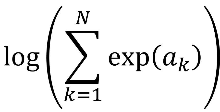
Sometimes you’ll need to calculate a sum of the form, $\sum_{k} \exp\left ( a_{k}\right )$ , where you have values for the $a_{k}$ . Really? Will you? Yes, it will probably be calculating a log-likelihood, or a contribution to a log-likelihood, so the actual calculation you want to do is of the form,

$\log\left ( \sum_{k} \exp \left ( a_{k}\right )\right )$

These sorts of calculations arise where you have log-likelihood or log-probability values $a_{k}$ for individual parts of an overall likelihood calculation. If you come from a physics calculation you’ll also recognise the expression above as the calculation of a log-partition function.

So what we need to do is exponentiate the $a_{k}$ values, sum them, and then take the log at the end. Hence the expression “log-sum-exp”. But why a blogpost on “log-sum-exp”? Surely, it’s an easy calculation. It’s just np.log(np.sum(np.exp(a))) , right ? Not quite.

It depends on the relative values of the $a_{k}$ . Do the naïve calculation np.log(np.sum(np.exp(a))) and it can be horribly inaccurate. Why? Because of overflow and underflow errors.

If we have two values $a_{1}$ and $a_{2}$ and $a_{1}$ is much bigger than $a_{2}$ , when we add $\exp(a_{1})$ to $\exp(a_{2})$ we are using floating point arithmetic to try and add a very large number to a much smaller number. Most likely we will get an overflow error. If would be much better if we’d started with $\exp(a_{1})$ and try to add $\exp(a_{2})$ to it. In fact, we could pre-compute $a_{2} - a_{1}$ , which would be very negative and from this we could easily infer that adding $\exp(a_{2})$ to $\exp(a_{1})$ would make very little difference. In fact, we could just approximate $\exp(a_{1}) + \exp(a_{2})$ by $\exp(a_{1})$ .

But how negative does $a_{2} - a_{1}$ have to be before we ignore the addition of $\exp(a_{2})$ ? We can set some pre-specified threshold, chosen to avoid overflow or underflow errors. From this, we can see how to construct a little Python function that takes an array of values $a_{1}, a_{2},\ldots, a_{N}$ and computes an accurate approximation to $\sum_{k=1}^{N}\exp(a_{k})$ without encountering underflow or overflow errors.

In fact we can go further and approximate the whole sum by first of all identifying the maximum value in an array $a = [a_{1}, a_{2}, \ldots, a_{N}]$ . Let’s say, without loss of generality, the maximum value is $a_{1}$ . We could ensure this by first sorting the array, but it isn’t necessary actually do this to get the log-sum-exp trick to work. We can then subtract $a_{1}$ from all the other values of the array, and we get the result,

$\log \left ( \sum_{k=1}^{N} \exp \left ( a_{k} \right )\right )\;=\; a_{1} + \log \left ( 1\;+\;\sum_{k=2}^{N} \exp \left ( a_{k} - a_{1} \right )\right )$

The values $a_{k} - a_{1}$ are all negative for $k \ge 2$ , so we can easily approximate the logarithm on the right-hand side of the equation by a suitable expansion of $\log (1 + x)$ . This is the “log-sum-exp” trick.

The great news is that this “log-sum-exp” calculation is so common in different scientific fields that there are already Python functions written to do this for us. There is a very convenient “log-sum-exp” function in the SciPy package, which I’ll demonstrate in a moment.

The log-sum-exp function

The sharp-eyed amongst you may have noticed that the last formula above gives us a way of providing upper and lower bounds for the ${\rm max}$ function. We can simply re-arrange the last equation to get,

${\rm max} \left ( a_{1}, a_{2},\ldots, a_{N} \right ) \;\le\; \log \left ( \sum_{k=1}^{N}\exp \left ( a_{k}\right )\right )$

The logarithm calculation on the right-hand side of the inequality above is what we call the log-sum-exp function (lse for short). So we have,

${\rm max} \left ( a_{1}, a_{2},\ldots, a_{N} \right ) \;\le\; {\rm lse}\left ( a_{1}, a_{2}, \ldots, a_{N}\right )$

This gives us an upper bound for the ${\rm max}$ function. Since $a_{k} \le {\rm max}\left ( a_{1}, a_{2},\ldots,a_{N}\right )$ , it is also relatively easy to show that,

${\rm lse} \left ( a_{1}, a_{2}, \ldots, a_{N}\right )\;\le\; {\rm max}\left ( a_{1}, a_{2},\ldots, a_{N} \right )\;+\;\log N$

and so we have have a lower bound for the ${\rm max}$ function. So the log-sum-exp function allows us to compute lower and upper bounds for the maximum of an array of real values, and it can provide an approximation of the maximum function. The advantage is that the log-sum-exp function is smooth and differentiable. In contrast, the maximum function itself is not smooth nor differentiable everywhere, and so is less convenient to work with mathematically. For this reason the log-sum-exp is often called the “real-soft-max” function because it is a “soft” version of the maximum function. It is often used in machine learning settings to replace a maximum calculation.

Calculating log-sum-exp in Python

So how do we calculate the log-sum-exp function in Python. As I said, we can use the SciPy implementation which is in scipy.special. All we need to do is pass an array-like set of values $a_{k}$ . I’ve given a simple example below,

			
# import the packages and functions we need
import numpy as np
from scipy.special import logsumexp
# create the array of a_k values 
a = np.array([70.0, 68.9, 20.3, 72.9, 40.0])
# Calculate log-sum-exp using the scipy function 
lse = logsumexp(a)
# look at the result
print(lse)

		

This will give the result 72.9707742189605

The example above and several more can be found in the Jupyter notebook DataScienceNotes2_LogSumExp.ipynb in the GitHub repository https://github.com/dchoyle/datascience_notes

The great thing about the SciPy implementation of log-sum-exp is that it allows us to include signed scale factors, i.e. we can compute,

$\log \left ( \sum_{k=1}^{N} b_{k}\exp\left ( a_{k}\right ) \right )$

where the values $b_{k}$ are allowed to be negative. This means, that when we are using the SciPy log-sum-exp function to perform the log-sum-exp trick, we can actually use it to calculate numerically stable estimates of sums of the form,

$\log \left ( \exp\left ( a_{1}\right ) \;-\; \exp\left ( a_{2}\right ) \;-\;\exp\left ( a_{3}\right )\;+\;\exp\left ( a_{4}\right )\;+\ldots\; + \exp\left ( a_{N}\right )\right )$ .

Here’a small code snippet illustrating the use of the scipy.special.logsumexp with signed contributions,

			
# Create the array of the a_k values
a = np.array([10.0, 9.99999, 1.2])
b = np.array([1.0, -1.0, 1.0])
# Use the scipy.special log-sum-exp function
lse = logsumexp(a=a, b=b)
# Look at the result
print(lse)

		

This will give the result 1.2642342014146895.

If you look at the output of the example above you’ll see that the final result is much closer to the value of the last array element $a_{3} = 1.2$ . This is because the first two contributions, $\exp(a_{1})$ and $\exp(a_{2})$ almost cancel each other out because the contribution $\exp(a_{2})$ is pre-fixed by a factor of -1. What we get left with is something close to $\log(\exp(a_{3}))\;=\; a_{3}$ .

There is also a small subtlety in using the SciPy logsumexp function with signed contributions. If the substraction of some terms had led to an overall negative result, scipy.special.logsumexp will rerturn NaN as the result. In order to get it to always return a result for us, we have to tell it to return the sign of the final summation as well, by setting the return_sign argument of the function to True. Again, you can find the code example above and others in the notebook DataScienceNotes2_LogSumExp.ipynb in the GitHub repository https://github.com/dchoyle/datascience_notes.

When you are having to combine lots of different probabilities, that are on very different scales, and you need to subtract some of them and add others, the SciPy log-sum-exp function is very very useful.

A Bland-Altman plot of the peak expiratory flow rate data taken from the 1986 Lancet paper of Bland and Altman.

Data Science Notes: 1. Bland-Altman plots

On December 6, 2025January 31, 2026 By dchoyleIn Data Science, Data Science Notes, Data Visualization1 Comment

Introduction

Summary: If you are using a scatter plot to compare two datasets, rotate your data.

Three times in the last six months I’ve explained to different colleagues and former colleagues what a Bland-Altman (BA) plot is. Admittedly, the last of those explanations was because I remarked to a colleague that I’d been talking about BA-plots and they then wanted to know what they were.

BA-plots are a really simple idea. I like them because they highlight how a human’s ability to perceive patterns in data can be markedly affected by relatively small changes in how that data is presented; rotating the data in this case.

I also like them because they are from the statisticians Martin Bland and Doug Altman who produced a well-known series of short articles, “Statistics Notes”, in the BMJ in the 1990s. Each article focused on a simple, basic, but very important statistical concept. The series ran over nearly 70 articles and the idea was to explain to a medical audience about ‘statistical thinking’. You can find the articles at Martin Bland’s website here. Interestingly, BA-plots were not actually part of this series of BMJ articles as their work on BA-plots had been published in earlier articles. However, I’d still thoroughly recommend having a browse of the BMJ series.

Since I’ve had to explain BA-plots three times recently, I thought I’d give it another go in a blogpost. Also, inspired by the Bland-Altman series, I’m going to attempt a series of 10 or so short blogposts on simple, basic Data Science techniques and concepts that I find useful and/or interesting. The main criterion for inclusion in my series is whether I think I can explain it in a short post, not whether I think it is important.

What is a Bland-Altman plot?

BA-plots are used for comparing similar sets of data. The original use-case was to test how reproducible a process was. Take two samples of data that ideally you would want to be identical and compare them using a BA plot. This could be comparing clinical measurements made by two different clinicians across the same set of patients. What we want to know is how reproducible is a clinical measurement if made by two different clinicians.

Perhaps the first way of visually comparing two datasets on the same objects would be to just do a scatter plot – one dataset values on the x-axis, the other dataset values on the y-axis. I’ve got an example in the plot below. In fact, I’ve taken this data from Bland and Altman’s original 1986 Lancet paper. You can see the plotted points are pretty close to the 45-degree line (shown as a black dashed line), indicating the two datasets are measuring the same thing with some scatter, perhaps due to measurement error.

A scatter plot of peak expiratory flow rate data taken from the original Bland Altman paper in the Lancet from 1986. — Scatter plot of original Bland Altman PEFR data

Now, here’s the neat idea. I can do exactly the same plot, but I’m just going to rotate it clockwise by 45-degrees. A little bit of high-school/college linear algebra will convince you that I can do that by creating two new features,

$\frac{1}{\sqrt{2}} \left ( y + x \right )$
$\frac{1}{\sqrt{2}} \left ( y - x \right )$

Here $x$ and $y$ are our starting features or values from the two datsets we are comparing. Typically, the pre-factors of $\sqrt{2}$ are omitted and we simply define our new features as,

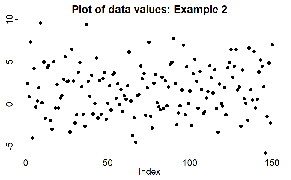
$A = \frac{1}{2} \left ( y + x \right )$
$M = \left ( y - x \right )$

Now we plot $M$ against $A$ . I’ve shown the new plot below.

Now a couple of things become clearer. Firstly, $A$ is the mean of $x$ and $y$ and so it gives us a better estimate of any common underlying value than just $x$ on its own or $y$ on its own. It gives us a good estimate of the size of the ‘thing’ we are interested in. Secondly, $M$ is the difference between $x$ and $y$ . $M$ tells us how different $x$ and $y$ are. Plotting $M$ against $A$ as I’ve done above shows me how reproducible the measurement is because I can easily see the scale of any discrepancies against the new vertical axis. I also get to see if there is any pattern in the level of discrepancy as the size of the ‘thing’ varies on the new horizontal axis. This was the original motivation for the Bland-Altman plot – to see the level of discrepancy between two sets of measurements as the true underlying value changes.

What the eye doesn’t see

What I really like about BA-plots though, is how much easier I find it to pick out if there is any systematic pattern to the differences between the two datasets. I haven’t looked into the psychological theory of visual perception, but it makes sense to me that humans would find it easier looking for differences as we move our eyes across one dimension – the horizontal axis – compared to moving our eyes across two dimensions – both the horizontal and vertical axes – when trying to scan the 45-degree line.

I first encountered BA-plots 25 years ago in the domain of microarray analysis. In that domain they were referred to as MA-plots (for obvious reasons). The choice of the symbols $M$ and $A$ also had a logic behind it. $M$ and $A$ are constructed as linear combinations of $x$ and $y$ , and in this case we “Add” them when constructing $A$ and “Minus” them when constructing $M$ . Hence the symbols $M$ and $A$ even tell you how to calculate the new features. You will also see BA-plots referred to Tukey mean-difference plots (again for obvious reasons).

In microarray analysis we were typically measuring the levels of mRNA gene expression in every gene in an organism across two different environmental conditions. We expected some genes to show differences in expression and so a few data points were expected to show deviations from zero on the vertical $M$ -axis. However, we didn’t expect broad systematic differences across all the genes, so we expected a horizontal data cloud on the MA-plot. Any broad systematic deviations from a horizontal data cloud were indicative of a systematic bias in the experimental set-up that needed to be corrected for. The MA plots gave an easy way to both visually detect any bias but also suggested an easy way to correct it. To correct it we just needed to fit a non-linear trendline through the data cloud, say using a non-parametric fit method like lowess. The vertical difference between a datapoint and the trendline was our estimate of the bias-corrected value of $M$ for that datapoint.

To illustrate this point I’ve constructed a synthetic example below. The left-hand plot shows the raw data in a standard scatterplot. The scatterplot suggests there is good agreement between the two samples – maybe a bit of disagreement but not much. However, when we look at the same data as a Bland-Altman plot (right-hand plot) we see a different picture. We can clearly see a systematic pattern to the discrepancy between the two samples. I’ve also estimated this systematic variation by fitting a non-linear trendline (in red) using the lowess function in the Python statsmodels package.

Two plots. The left hand plot shows a standard scatterplot, whilst the right-hand plot shows the corresponding Bland-Altman plot. — Scatterplot and Bland-Altman plot for the second example dataset.

Sometimes we may expect a global systematic shift between our paired data samples, i.e. a constant vertical shift on the $M$ axis. Or at least we can explain/interpret such a shift. Or there may be other patterns of shift we can comfortably interpret. This widens the applications domains we can use BA-plots for. In commercial Data Science I’ve seen BA-plots used to assess reproducibility of metrics on TV streaming advertising, and also calibration of transaction data across different supermarket stores. Next time you’re using a vanilla scatterplot to compare two data series, think about rotating and making a BA-plot.

All the code for the examples I’ve given in this post is in the Jupyter notebook DataScienceNotes1_BlandAltmanPlots.ipynb which can be found in the public GitHub repository https://github.com/dchoyle/datascience_notes. Feel free to clone the repository and play with the notebook. I’ll be adding to the repository as I add further “Data Science Notes” blogposts.

Hoyle Analytics

Category: Data Science Notes

Data Science Notes: 5. Trimmed variances and getting MAD

Summary

Introduction

Theory

Practice

Getting MAD

Other distributions

Conclusions

Data Science Notes: 4. What is an outlier?

Summary

Introduction

What do you think an outlier is?

An illustration

Life (and data) is always made up of multiple processes

How to detect outliers?

Conclusions

Data Science Notes: 2. Log-Sum-Exp

Summary

Introduction

The log-sum-exp trick

The log-sum-exp function

Calculating log-sum-exp in Python

Data Science Notes: 1. Bland-Altman plots

Introduction

What is a Bland-Altman plot?

What the eye doesn’t see

Summary

Introduction

Theory

Practice

Getting MAD

Other distributions

Conclusions

Share this:

Summary

Introduction

What do you think an outlier is?

An illustration

Life (and data) is always made up of multiple processes

How to detect outliers?

Conclusions

Share this:

Summary

Introduction

The log-sum-exp trick

The log-sum-exp function

Calculating log-sum-exp in Python

Share this:

Introduction

What is a Bland-Altman plot?

What the eye doesn’t see

Share this:

Share this: