Using your own algorithms with hyperparameter optimization in AWS SageMaker

TL;DR

AWS SageMaker provides a number of standard Machine Learning algorithms in containerized form, so you can pull those algorithms down onto a large EC2 instance and just run, with minimal effort.
AWS SageMaker also provides a hyperparameter optimization functionality that pretty much runs ‘out-of-the-box’ with the algorithms provided.
You can run your own algorithms within SageMaker if you containerize your algorithm code.
I wanted to find out if it was possible to easily combine the ‘run-your-own-containerized-algorithm’ functionality with the ‘out-the-box’ hyperparameter optimization functionality in SageMaker. It is. It was a straight-forward, but slightly lengthy process.

Introduction

<DISCLAIMER> This is a blog-post I started back in Autumn/Winter 2019. I knew it would be a fairly length post but one I was keen to write. But then, well, a pandemic got in the way and its taken a while to get back to writing blog posts. I still believe there are some useful learnings here – I hope you do too </DISCLAIMER>.

Back in 2019 I was using SageMaker a lot, including running an AWS Machine Learning Immersion Day at Infinity Works. One of the things I like about SageMaker is how the resources used to do any heavy lifting in training a model are separated from the resources supporting the Jupyter notebook. The SageMaker service provides several standard Machine Learning algorithms (e.g. Random Forests, XGBoost) in containers. This means it is possible to explore a dataset and develop an modelling approach in a Jupyter notebook that runs on one EC2 instance, and then when we want to scale-up the training process to the full dataset we can pull down the relevant container from ECR and run the training process on a separate much larger instance. Provisioning of heavier infrastructure needed for training on the full large dataset is only done when it is needed and you only pay for what you use of those larger EC2 instances. A Data Scientist like me doesn’t have to worry about the provisioning of the larger EC2 instance, it is handled by through simple configuration options when configuring the training job. It is also possible to configure a hyper-parameter optimization job in a similar way, so that multiple training jobs (with different hyper-parameter values) can be easily run, potentially in parallel, on large EC2 instances just by adjusting a few lines of json config.

So far, so good. As a Data Scientist the pain of getting access to or configuring compute resource has been removed and training on really large datasets is almost as easy as exploring a smaller dataset in a Jupyter notebook running on my local machine. But are we restricted to only using the algorithms that AWS has containerized? This is where it get more interesting and fun. You can use any algorithm that is available in a container in ECS. That means you can develop/code up your own algorithm/training process, containerize it, and then run that algorithm using multiple large EC2 instances with minimal config.

AWS have an example of how to containerize your own algorithm and deploy it to an endpoint. The git repo is here. The AWS team use the example of a scikit-learn decision tree trained on the Iris dataset (I know, why do examples not use something more original than the Iris dataset).

What I wanted to explore was,

How easy was it to actually containerize my own algorithm for use in SageMaker,
How easy was it to combine my containerized algorithm with the easy to configure hyperparameter optimization capability already present in SageMaker.

The rest of this post is about what I learnt in exploring those two questions, in particular the second of those. The first question is essentially already answered by the original AWS repo. What I wanted to learn was could I easily use my own algorithm with the out-the-box hyperparameter optimization functionality that SageMaker provided, or was the easy-to-use hyperparameter optimization functionality essentially restricted to the in-built SageMaker algorithms? What I’ll cover is,

The choice of algorithm we’re going to containerize
The basics of building the Docker container
Pushing the container to the AWS container registry
Using the containerized algorithm within a SageMaker notebook
Running hyperparameter optimization jobs using the containerized algorithm.

If you want to follow the technical details, I would suggest that you first become familiar with the basics of AWS SageMaker – tutorial here. You may also want to look at the basics of hyperparameter tuning for one of the standard machine learning algorithms within SageMaker, as I’ll be assuming some of this background knowledge is known to you or at least you can pick it up quickly – to fully explain all the SageMaker background material would make this an even longer blog. You can find explanations of how to configure and run a SageMaker hyperparameter tuning job here and here.

Now, let’s start with the first of our questions.

Algorithm choice

I wanted to use an algorithm that wasn’t already available within SageMaker, otherwise what would be the point of going through this exercise? I have been doing some work recently on Gaussian Processes (GPs), in particular with kernel functions that are composite functions.

I won’t explicitly cover the basics of GPs here – the blog post is long enough already. Instead I will point you towards the excellent book by Carl Rasmussen and Chris Williams and this tutorial from Neil Lawrence. However, I will say briefly what my interest in GPs is. Gaussian Processes have an interesting connection with large (wide) Neural Networks. This connection was discovered by Chris Williams and Radford Neal. I wrote some GP code, on the basis of the Williams’ paper, that made it into commercial software (my first ever example) back in 1999 (yes – I am that old, and have been working in Machine Learning that long). More recently, the connection has been extended to link Deep Learning Neural Networks and Gaussian Processes (see for example, here and here). Cho & Saul did some nice early work in this area, using dot-product kernels that are composite functions. It is the dot-product kernels derived by Cho & Saul that I’ll use here for my example algorithm, as the kernels are of relatively simple form, and yet are specified in terms of a few simple parameters that we can regard as hyper-parameters. For the purposes of this blog on AWS SageMaker it is not important to know what the Cho & Saul kernels might represent, merely how they are defined mathematically. So let’s start there,

For this illustration we are focusing on datapoints on the the surface of the unit hypersphere, i.e ${\bf x} \in \mathbb{R}^{d}$ with $||{\bf x}||_{2}^{2}\;=\;1$ . We then consider a set of kernels, $K_{q,l}\left ( {\bf x}_{1}, {\bf x}_{2} \right)$ , defined via,

$K_{q,l}\left ({\bf x}_{1}, {\bf x}_{2} \right )\;=\; k_{q,l}\left ( {\bf x}_{1}\cdot {\bf x}_{2} \right )$

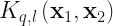
The dot-product kernels $k_{q,l}(t)$ are defined iteratively,

$k_{q,l+1}(t)\;=\;k_{q,0}\left ( k_{q, l}(t)\right )$

The base kernels $k_{q,0}(t)$ are constructed from,

$k_{q,0}(t)\;=\; J_{q}\left ( \arccos (t)\right ) / J_{q}\left ( 0\right )$

with,

$J_{q}\left ( \theta \right )\;=\;(-1)^{q}\left (\sin\theta\right)^{2q+1}\left ( \frac{1}{\sin\theta}\frac{\partial}{\partial \theta}\right )^{q} \left ( \frac{\pi-\theta}{\sin\theta}\right )$

Choosing a particular kernel then boils down to making a choice for q and l. Once we have made choice of kernel, we can train our model. For simplicity, I have defined the model training here to be simply the process of constructing the Gram matrix from the training data, i.e. the process of calculating the matrix elements,

$M_{ij} = \sigma^{2}\delta_{ij}\;+\;K_{q,l}\left ( {\bf x}_{i}, {\bf x}_{j}\right)$

Here, σ² is the variance of the additive Gaussian noise that we consider present in the response variable, and 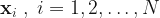${\bf x}_{i}\;,\; i=1,2,\ldots,N$ , are the feature vectors for the N datapoints in the training set. Along with the training feature vectors we also have the response variable values, $y_{i}$ .

Whilst it may not match the more traditional concept of model training – there is no iterative process to minimize some cost function – I am using the training data to construct a mathematical object required for calculating the expectation of the response variable conditional on the input features. Within a Gaussian Process it is considered usual to optimize any parameters of the covariance kernel as part of the model training. In this case, for simplicity, and for purposes of illustrating the hyperparameter tuning capabilities of SageMaker, I wanted to consider the kernel parameters q,l and σ² as hyperparameters, essentially leaving no remaining kernel parameters to be optimized during the model training.

Once we have the matrix ${\bf M}$ defined, we can calculate a prediction for the response variable at a new feature vector ${\bf x}_{\star}$ via the formula,

$\mathbb{E}\left ( y\left ( {\bf x}_{\star}\right )\right )\;=\;{\bf v}\left ( {\bf x}_{\star}\right )^{\top}{\bf M}^{-1}{\bf y}\,\,$

where ${\bf y}$ is the vector of response values in the training set, and the vector ${\bf v}\left ( {\bf x}_{\star} \right )\;=\; (v_{1}, v_{2}, \ldots, v_{N})$ , with the element $v_{i}\left ( {\bf x}_{\star}\right )$ given by,

$v_{i}\;=\; k_{q,l}\left ( {\bf x}_{\star}\cdot {\bf x}_{i}\right )$

Now we have given the mathematical definition of our algorithm, we need to focus on code. Following the example in the original AWS repo we need python code that,

Defines a class for a trained GP model. I have called my class, unsurprisingly, trainedGPModel . Instantiating an instance of this class by passing the training data to the class constructor method, runs the Gram matrix calculation process mentioned earlier. Within my trainedGPModel class I also have a method predict(xstar) that returns the predicted expectation of the response variable given an input datapoint xstar. The code for the trainedGPModel class implements the linear algebra formulae given above and so is straight-forward.
We also need code that runs the training process. This code is held in a file called train. I made minimal modifications to the train module in the original AWS repo. The main change I made was including code to make predictions on a validation dataset, and from that calculating the Root-Mean-Squared-Error (RMSE) on the validation dataset. The validation RMSE is the metric I will use for hyperparameter tuning and so I have to write the validation RMSE value to stdout so that it can get picked up by the SageMaker hyperparameter tuning process. I had to write the RMSE value with a string prefix and delimiter, e.g.

print( "validation:RMSE=" + str(RMSE_validation) + ";" )

with a corresponding matching regex in the configuration of the hyperparameter tuning job – see later section on running the containerized algorithm in a SageMaker notebook. It wasn’t obvious that I needed to write the validation metric in this way, and it took a bit of googling to work out. Most SageMaker links on hyperparameter tuning point to this page , but the detail on how the metric is passed between your algorithm code and the SageMaker hyperparameter optimization code is actually explained in this SageMaker documentation page.

Docker basics

Now let’s talk about putting our code in a container. We need to construct a Docker compose file. For a refresher on Docker I found this tutorial by Márk Takács to be really helpful. I actually use a Windows machine for my work, so I’m running Docker Desktop. However, I also use WSL (Windows Subsystem for Linux) for when I want a linux like environment. Although you can install a Docker client under WSL, you still have to make use of the native Docker daemon of Docker Desktop. I found this guide from Nick Janetakis on getting the WSL Docker client working with Docker Desktop invaluable, particularly the configuring of where WSL mounts the Windows file system (by editing the /etc/wsl.config file) so that I can then easily mount any sub-directory of my Windows file system to any point I choose in the container image when testing the Docker file locally.

I won’t go through the aspects of testing the container locally – you can read the original AWS repo to see that. Instead we’ll just go through the Docker file for building the final SageMaker container. The Docker file is fairly simple and other that changing it to use a python3 runtime (see lines 9&10) we have not changed anything else in the Docker file in the original AWS repo. Line 36 of the Docker file is where we copy across our algorithm code into pre-specified directory in the image that SageMaker will look for when running the containerized algorithm.


# Build an image that can do training and inference in SageMaker
# This is a Python 3 image that uses the nginx, gunicorn, flask stack
# for serving inferences in a stable way.

FROM ubuntu:18.04

RUN apt-get -y update && apt-get install -y --no-install-recommends \
wget \
python3 \
python3-pip \
nginx \
ca-certificates \
&& rm -rf /var/lib/apt/lists/*

# Here we get all python packages.
# There's substantial overlap between scipy and numpy that we eliminate by
# linking them together. Likewise, pip leaves the install caches populated which uses
# a significant amount of space. These optimizations save a fair amount of space in the
# image, which reduces start up time.
RUN pip3 install numpy scipy scikit-learn pandas flask gevent gunicorn &amp;amp;&amp;amp; \
(cd /usr/local/lib/python3.6/dist-packages/scipy/.libs; rm *; ln ../../numpy/.libs/* .) && \
rm -rf /root/.cache

RUN pip3 install setuptools

# Set some environment variables. PYTHONUNBUFFERED keeps Python from buffering our standard
# output stream, which means that logs can be delivered to the user quickly. PYTHONDONTWRITEBYTECODE
# keeps Python from writing the .pyc files which are unnecessary in this case. We also update
# PATH so that the train and serve programs are found when the container is invoked.

ENV PYTHONUNBUFFERED=TRUE
ENV PYTHONDONTWRITEBYTECODE=TRUE
ENV PATH="/opt/program:${PATH}"

# Set up the program in the image
COPY gaussian_processes /opt/program
WORKDIR /opt/program

Pushing the container to AWS

We can now push our Docker container to the AWS ECR (Elastic Container Registry). This is simple using the AWS CLI (command line interface) and the build_and_push.sh shell script provided in the original AWS repo. Within the shell script we have just modified on lines 16 and 17 the name of the top-level directory in which our training and prediction code resides,

image=$1

if [ "$image" == "" ]
then
    echo "Usage: $0 "
    exit 1
fi

chmod +x gaussian_processes/train
chmod +x gaussian_processes/serve

Then we just run shell script, passing the name of the container we have just built as a command line argument,

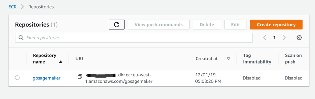
./build_and_push.sh gpsagemaker

After running the shell script we can see the container present in the AWS ECR,

Screenshot of our Gaussian Process SageMaker Docker container in AWS Elastic Container Registry (ECR) – ready to use within a SageMaker notebook.

Using the containerized algorithm in SageMaker

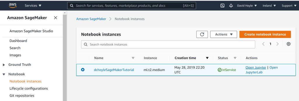
Now we have the container, that has our GP code, in AWS ECR we can use it within a SageMaker notebook. Let’s do so. For this I’m just going to adapt the notebook within the original AWS repo. I go to the Sagemaker under ‘ML’ in the list of AWS services and from there I can start/create my SageMaker notebook instance. Once the notebook instance is ready I can open up a Jupyter notebook as usual,

The first main difference is that we’ll create some simple small-scale simulated training and validation data. Our goal here is to test how easy it is to containerize and use our own algorithm, not build a perfect model. Our generative model is a simple one – a linear model, dependent on just two features (with coefficients that we have chosen as 1.5 and 5.2 respectively). We use this simple model to create the response variable values and then add some Gaussian random noise (of unit variance).


# create training and validation sets
nTrain = 100
X_train = np.random.randn( nTrain, 2 )
y_train = (1.5 * X_train[:, 0]) + (5.2*X_train[:,1]) + np.random.randn( nTrain )
y_train.shape = (nTrain, 1)
data_train = np.concatenate( (y_train, X_train), axis=1)
df_data_train = pd.DataFrame( data_train )

nValidation = 50
X_validation = np.random.randn( nValidation,2 )
y_validation = (1.5 * X_validation[:, 0]) + (5.2*X_validation[:,1]) + np.random.randn( nValidation )
y_validation.shape = ( nValidation, 1 )
data_validation = np.concatenate( (y_validation, X_validation), axis=1)
df_data_validation = pd.DataFrame( data_validation )

We then specify our account details and also the image that contains our Gaussian Process algorithm.


account = boto3.client('sts').get_caller_identity()['Account']
region = boto3.session.Session().region_name
image = '{}.dkr.ecr.{}.amazonaws.com/gpsagemaker:latest'.format(account, region)

The next cell in our notebook then uploads the training and validation data to our s3 bucket,


# write training and validation sets to s3
from io import StringIO # python3; python2: BytesIO 
import boto3

bucket = mybucket

# write training set
csv_buffer = StringIO()
df_data_train.to_csv(csv_buffer, header=False, index=False)
s3_resource = boto3.resource('s3')
s3_resource.Bucket(bucket).Object('train/train_data.csv').put(Body=csv_buffer.getvalue())
csv_buffer.close()

# write validation set
csv_buffer = StringIO()
df_data_train.to_csv(csv_buffer, header=False, index=False)
s3_resource = boto3.resource('s3')
s3_resource.Bucket(bucket).Object('validation/validation_data.csv').put(Body=csv_buffer.getvalue())
csv_buffer.close()

Running a single training job

So first of all let’s just configure and run a single simple training job. Note the validation metric being specified along with the regex.


create_training_params = \
{
    "RoleArn": role,
    "TrainingJobName": job_name,
    "AlgorithmSpecification": {
        "TrainingImage": image,
        "TrainingInputMode": "File",
        "MetricDefinitions":[{"Name":"validation:RMSE",
                              "Regex":"validation:RMSE=(.*?);"    
        }]
    },

We also set values for the hyperparameters, which are static since we are just running a single training job and not doing any hyperparameter optimization yet.


    "HyperParameters": {
        "q":"0",
        "l":"2",
        "noise":"0.1"
    },

We can then run a training job using our containerized Gaussian Process code, just as we would any other algorithm available in SageMaker. We can see the training job running in the AWS Management console – click under “Training jobs” on the left hand side of the console. We can see the current training job ‘in progress’ and also an earlier completed training job that I ran.

Screenshot of a single SageMaker training job running using our GP algorithm code.

Running a hyperparameter tuning job

So that appears to run ok. So now we have our algorithm running in SageMaker ok, we can now just configure the SageMaker hyperparameter optimization wrapper and run one of the out-of-box SageMaker hyperparameter optimization algorithms over what we have specified as hyperparameter in our Gaussian Process code. The config for the hyperparameter tuning job is below – we have largely just modified slightly the examples in the original AWS repo and also followed the guidance. You can see that we have specified the RMSE metric on the validation set as the metric to optimize with respect to the hyperparameters. For illustration purposes we have specified that we want to optimize only over the q and l hyperparameters. The σ² hyperparameter we have kept static at σ²=0.1. You can also see that we have specified to run 10 training jobs in total, i.e. we will evaluate the validation metric at 10 different combinations of the two hyperparameters, but we only run 3 training jobs in parallel at any one time.


# Define HyperParameterTuningJob
# We will only tune the learning rate by maximizing the AUC value of the 
# validation set. The hyperparameter search is a random one, using a sample of
# 10 training jobs - better methods for searching the hyperparameter space are 
# available, but for simplicty and demonstration purposes we will use the 
# random search method. Run a max of 3 training jobs in parallel
job_name = "gpsmbyo-hp-" + strftime("%Y-%m-%d-%H-%M-%S", gmtime())
response = sm.create_hyper_parameter_tuning_job(
    HyperParameterTuningJobName=job_name,
    HyperParameterTuningJobConfig={
        'Strategy': 'Random',
        'HyperParameterTuningJobObjective': {
            'Type': 'Minimize',
            'MetricName': 'validation:RMSE'
        },
        'ResourceLimits': {
            'MaxNumberOfTrainingJobs': 10,
            'MaxParallelTrainingJobs': 3
        },
        'ParameterRanges': {
            'IntegerParameterRanges': [
            {
              "Name": "q",
              "MaxValue": "4",
              "MinValue": "0",
              "ScalingType": "Auto"
            },
            {
              "Name": "l",
              "MaxValue": "4",
              "MinValue": "1",
              "ScalingType": "Auto"
            }    
        ]}
    },
    TrainingJobDefinition={
        'StaticHyperParameters': {
            "noise":"0.1"
        },
        'AlgorithmSpecification': {
        'TrainingImage': image,
        'TrainingInputMode': "File",
        'MetricDefinitions':[{"Name":"validation:RMSE",
                              "Regex":"validation:RMSE=(.*?);"
                             }]
        }

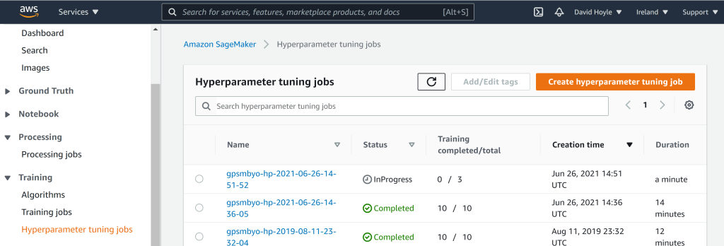
If we then look at our AWS console (screenshot below) we can see the hyperparameter tuning job running, along with previous completed tuning jobs.

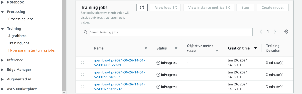
Screen shot of AWS console showing current and previous hyperparameter tuning jobs.

We can also see the individual training jobs, corresponding to that tuning job, running (screenshot below). Remember that the hyperparameter tuning job is just a series of individual evaluations of the validation metrics, run at combinations of (q,l) specified the tuning algorithm. From the screenshot we can see that there are 3 training jobs running, in accordance with what we specified in the tuning job config.

Screenshot of the 3 training jobs running as part of the hyperparameter tuning job.

Once the tuning job has completed, we can retrieve the validation metric values for the 10 different hyperparameter combinations that were tried, to see which combination of q and l gave the smallest RMSE on the validation set.

Summary

The two questions I was trying to address were,

How difficult is it to create your own algorithm to use in SageMaker?
How easy is it to use the hyperparameter optimization algorithms available in SageMaker with your new algorithm?

The answer to both questions is, “it is a relatively easy but lengthy process”. That it is a lengthy process is understandable – SageMaker gives you a functionality to apply out-the-box hyperparameter tuning on an algorithm/code that it knows nothing about until runtime. Therefore there has to be a lot of standardized syntax in specifying how that algorithm is structured and called as a piece of code. Fortunately, all the details of how to structure your algorithm and create the Docker container are in the excellent example given in the AWS repo and the documentation. The only complaint I would have is that it would be good for the repo to have an example showing how your own algorithm can utilize the hyperparameter optimization functionality of SageMaker – hence this blog. Working out the few remaining steps to get the hyperparameter optimization working with my Gaussian Process code was not very difficult, but not easy either.

The example algorithm I have chosen is very simplistic – the training process literally only involves the calculation and inversion of a matrix. A full training process could involve optimization of, say, the log-likelihood with respect to the parameters of the kernel function, but explaining the extra details would make this blog even long. Secondly, we only needed a simple/minimal training process to address the two questions above. Likewise, we have not illustrated our new trained algorithm being used to serve predictions – this is very well illustrated in the original repo and I would not be adding any new with my Gaussian Process example.

Hoyle Analytics

Using your own algorithms with hyperparameter optimization in AWS SageMaker

TL;DR

Introduction

Algorithm choice

Docker basics

Pushing the container to AWS

Using the containerized algorithm in SageMaker

Running a single training job

Running a hyperparameter tuning job

Summary

Leave a Reply Cancel reply

TL;DR

Introduction

Algorithm choice

Docker basics

Pushing the container to AWS

Using the containerized algorithm in SageMaker

Running a single training job

Running a hyperparameter tuning job

Summary

Share this:

Like this:

Leave a Reply Cancel reply