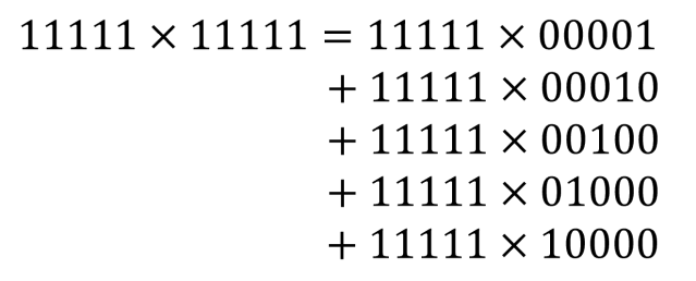
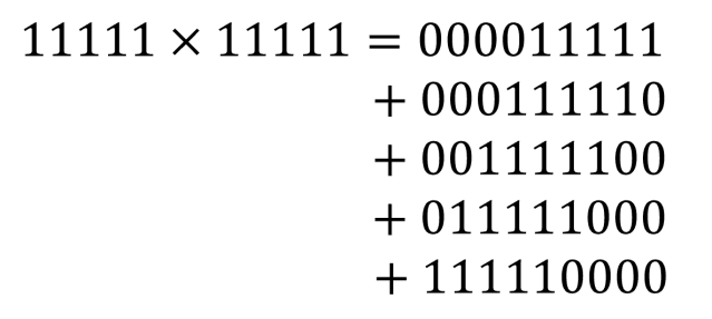
Before Christmas I set a little puzzle. The challenge was to calculate the proportion of file sizes on your hard drive that start with the digit 1. I predicted that the proportion you got was around 30%. I’ll now explain why.
Benford’s Law
The reason why around 30% of all the file sizes on your hard disk start with 1 is because of Benford’s Law. Computer file sizes approximately follow Benford’s Law.
What is Benford’s Law?
Benford’s Law says that for many datasets the first digits of the numbers in the dataset follow a particular distribution. Under Benford’s Law, the probability of the first digit being equal to d is,
Eq.1
So, in a dataset that follows Benford’s Law, the probability that a number starts with a 1 is around 30%. Hence, the percentage of file sizes that start with 1 is around 30%.
The figure below shows a comparison of the distribution in Eq.1 and the distribution of first digits of file sizes for files in the “Documents” folder of my hard drive. The code I used to calculate the empirical distribution in the figure is given at the end of this post. You can see the distribution derived from my files is in very close agreement with the distribution predicted by Eq.1. The agreement between the two distributions in the figure is close but not perfect – more on that later.

Benford’s Law is named after Frank Benford, whose discovered the law in 1938 – see the later section for some of the long history of Benford’s Law. Because Benford’s Law is concerned with the distribution of first digits in a dataset, it is also commonly referred to as, ‘the first digit law’ and also the ‘significant digit law’.
Benford’s Law is more than just a mathematical curiosity or Christmas cracker puzzle. It has some genuine applications – see later. It has also fascinated mathematicians and statisticians because it applies to so many diverse datasets. Benford’s Law has been shown to apply to datasets as different as the size of rivers and election results.
What’s behind Benford’s Law
The intuition behind Benford’s Law is that if we think there are no a priori constraints on what value a number can take then we can make the following statements,
- We expect the numbers to be uniformly distributed in some sense – more on that in a moment.
- There is no a priori scale associated with the distribution of numbers. So, I should be able to re-scale all my numbers and have a distribution with the same properties.
Overall, this means we expect the numbers to be uniformly distributed on a log scale.
This intuition helps us identify when we should expect a dataset to follow Benford’s Law, and it also gives us a hand-waving way of deriving the form of Benford’s Law in Eq.1.
Deriving Benford’s Law
First, we restrict our numbers to be positive and derive Benford’s Law. The fact that Benford’s Law would also apply to negative numbers once we ignore their sign should be clear.
We’ll also have to restrict our positive numbers to lying in some range so that the probability distribution of
is properly normalized. We’ll then take the limit
at the end. For convenience, well take
to be of the form
, and so the limit
corresponds to the limit
.
Now, if our number lies in
and is uniformly distributed on a log-scale, then the probability density for
is,
The probability of getting a number between, say 1 and 2 is then,
Now numbers which start with a digit are of the form
with
and
. So, the total probability of getting such a number is,
and so after performing the integration and summation we have,
Recalling that we have chosen , we get,
Finally, taking the limit gives us Benford’s Law for positive valued numbers which are uniformly distributed on a log scale.
Ted Hill’s proof of Benford’s Law
The derivation above is a very loose (lacking formal rigour) derivation of Benford’s Law. Many mathematicians have attempted to construct a broadly applicable and rigorous proof of Benford’s Law, but it was not until 1995 that a widely accepted proof was derived by Ted Hill from Georgia Institute of Technology. You can find Hill’s proof here. Ted Hill’s proof also seemed to reinvigorate interest in Benford’s Law. In the following years there were various popular science articules on Benford’s Law, such as this one from 1999 by Robert Matthews in The New Scientist. This article was where I first learned about Benford’s Law.
Benford’s Law is base invariant
The approximate justification we gave above for why Benford’s Law works made no explicit reference to the fact that we were working with numbers expressed in base 10. Consequently, that justification would be equally valid if we were working with numbers expressed in base . This means that Benford’s Law is base invariant, and a similar derivation can be made for base
.
The distribution of first digits given in Eq.1 is for numbers expressed in base 10. If we express those same numbers in base and write a number
in base
as,
then the first digit is in the set
and the probability that the first digit has value
is given by,
Eq.2
When should a dataset follow Benford’s Law?
The broad intuition behind Benford’s Law that we outlined above also gives us an intuition about when we should expect Benford’s Law to apply. If we believe the process generating our data is not restricted in the scale of the values that can be produced and there are no particular values that are preferred, then a large dataset drawn from that process will be well approximated by Benford’s Law. These considerations apply to many different types of data generating processes, and so with hindsight it should not come as a surprise to us that many different datasets appear to follow Benford’s Law closely.
This requires that no scale emerges naturally from the data generating process. This means the data values shouldn’t be clustered around a particular value, or particular values. So, data drawn from a Gaussian distribution would not conform to Benford’s law. From the perspective of the underlying processes that produce the data, this means there shouldn’t be any equilibrium process at work, as that would drive the measured data values to the value corresponding to the equilibrium state of the system. Likewise, there should be no constraints on the system generating the data, as the constraints will drive the data towards a specific range of values.
However, no real system is truly scale-free. The finite system size always imposes a scale. However, if we have data that can vary over many orders of magnitude then from a practical point of view, we can regard that data as effectively scale free. I have found that data that varies over 5 orders of magnitude is usually well approximated by Benford’s law.
Because a real-world system cannot really ever truly satisfy the conditions for Benford’s Law, we should expect that most real-world datasets will only show an approximate agreement with Benford’s Law. The agreement can be very close, but we should still expect to see deviations from Benford’s Law – just as we saw in the figure at the top of this post. Since real-world datasets won’t follow Benford’s Law precisely, we also shouldn’t expect to see a real-world dataset follow the base-invariant form of Benford’s Law in Eq.2 for every choice of base. In practice, this means that there is usually a particular base for which we will see closer agreement with the distribution in Eq.2, compared to other choices of base.
Why computer file sizes follow Benford’s Law
Why does Benford’s Law apply to the sizes of the files on your computer? Those file sizes can span over several orders of magnitude – from a few hundred bytes to several hundred megabytes. There is also no reason why my files should cluster around a particular file size – I have photos, scientific and technical papers, videos, small memos, slides, and so on. It would be very unusual if all those different types of files, from different use cases, end up having very similar sizes. So, I expect Benford’s Law to be a reasonable description of the distribution of first digits of the file sizes of files in my “Documents” folder.
However, if the folder I was looking at just contained, say, daily server logs, from a server that ran very unexciting applications, I would expect the server log file size to be very similar from one day to the next. I would not expect Benford’s Law to be a good fit to those server log file sizes.
In fact a significant deviation from Benford’s Law in the file size distribution would indicate that we have a file size generation process that is very different from a normal human user going about their normal business. That may be entirely innocent, or it could be indicative of some fraudulent activity. In fact, fraud detection is one of the practical applications of Benford’s Law.
The history of Benford’s Law
Simon Newcomb
One of the reasons why the fascination with Benford’s Law endures is the story of how it was discovered. With such an intriguing mathematical pattern, it is perhaps no surprise to learn that Frank Benford was not the first scientist to spot the first-digit pattern. The astronomer Simon Newcomb had also published a paper on, “the frequency of use of the different digits in natural numbers” in 1881. Before the advent of modern computers, scientists and mathematicians computed logarithms by looking them up in mathematical tables – literally books of logarithm values. I still have such a book from when I was in high-school. The story goes that Newcomb noticed that in a book of logarithms the pages were grubbier, i.e. used more, for numbers whose first significant digit was 1. From this Newcomb inferred that numbers whose first significant digit was 1 must be more common, and he supposedly even inferred the approximate frequency of such numbers from the relative grubbiness of the pages in the book of logarithms.
In more recent years the first-digit law is also referred to as the Newcomb-Benford Law, although Benford’s Law is still more commonly used because of Frank Benford’s work in popularizing it.
Benford’s discovery
Frank Benford rediscovered the law in 1938, but also showed that data from many diverse datasets – from the surface area of rivers to population sizes of US counties – appeared to follow the distribution in Eq.1. Benford then published his now famous paper, “The law of anomalous numbers”.
Applications of Benford’s Law
There are several books on Benford’s Law. One of the most recent, and perhaps the most comprehensive is Benford’s Law: Theory and Applications. It is divided into 2 sections on General Theory (a total of 6 chapters) and 4 sections on Applications (a total of 13 chapters). Those applications cover the following:
- Detection of accounting fraud
- Detection of voter fraud
- Measurement of the quality of economic statistics
- Uses of Benford’s Law in the natural sciences, clinical sciences, and psychology.
- Uses of Benford’s Law in image analysis.
I like the book because it has extensive chapters on applications written by practitioners and experts on the uses of Benford’s Law, but the application chapters make links back to the theory.
Many of the applications, such as fraud detection, are based on the idea of detecting deviations from the Benford Law distribution in Eq.1. If we have data that we expect to span several orders of magnitude and we have no reasons to suspect the data values should naturally cluster around a particular value, then we might expect it to follow Benford’s Law closely. This could be sales receipts from a business that has clients of very different sizes and sells goods or services that vary over a wide range of values. Any large deviation from Benford’s Law in the sales recipts would then indicate the presence of a process that produces very specific receipt values. That process could be data fabrication, i.e. fraud. Note, this doesn’t prove the data has been fraudulently produced, it just means that the data has been produced by a process we wouldn’t necessarily expect.
My involvement with Benford’s Law
In 2001 I published a paper demonstrating that data from high-throughput gene expression experiments tended to follow Benford’s Law. The reasons why mRNA levels should follow Benford’s Law is ultimately those we have already outlined – mRNA levels can range over many orders of magnitude and there are no a priori molecular biology reasons why, across the whole genome, mRNA levels should be centered around a particular value.
In December 2007 a conference on Benford’s Law was organized by Prof. Steven Miller from Brown University and others. The conference was held in a hotel in Sante Fe and was sponsored/funded by Brown University, the University of New Mexico, Universidade de Vigo, and the IEEE. Because of my 2001 paper, I received an invitation to talk at the workshop.
For me, the workshop was very memorable for many reasons,
- I had a very bad cold at the time.
- Due to snow in both the UK and US, I was snowbound overnight in Chicago airport (sleeping in the airport), and only just made a connecting flight in Dallas to Albuquerque. Unfortunately, my luggage didn’t make the flight connection and ended up getting lost in all the flight re-arrangements and didn’t show up in Santa Fe until 2 days later.
- It was the first time I’d seen snow in the desert – this really surprised me. I don’t know why, it just did.
- Because of my cold, I hadn’t finished writing my presentation. So I stayed up late the night before my talk to finish writing my slides. To sustain my energy levels through the night whilst I was finishing writing my slides, I bought a Hershey bar thinking it would be similar to chocolate bars in the UK. I took a big bite from the Hershey bar. Never again.
- But this was all made up for by the fact I got to sit next to Ted Hill during the workshop dinner. Ted was one of the most genuine and humble scientists I have had the pleasure of talking to. Secondly, the red wine at the workshop dinner was superb.
From that workshop Steven Miller organized and edited the book on Benford’s Law I referenced above. Hence why I think that book is one of the best on Benford’s Law, although I am biased as I contributed one of the chapters – Chapter 16 on “Benford’s Law in the Natural Sciences”
My Python code solution
To end this post, I have given below the code I used to calculate the distribution of first digits of the file sizes on my laptop hard drive.
import numpy as np

# We'll use the pathlib library to recurse over
# directories
from pathlib import Path

# Specify the top level directory
start_dir = "C:\\Users\\David\\Documents"

# Use a list comprehension to recursively loop over all sub-directories
# and get the file sizes
filesizes = [path.lstat().st_size for path in list(Path(start_dir).glob('**/*' )) if path.is_file()]

# Now count how many file sizes start with a 1
proportion1 = np.sum([int(str(i)[0])==1 for i in filesizes])/len(filesizes)

# Print the result
print("Proportion of filesizes starting with 1 = " + str(proportion1))
print("Number of files = " + str(len(filesizes)))

# Calculate the first-digit proportions for all digits 1 to 9
proportions = np.zeros(9)
for i in range(len(filesizes)):
    proportions[int(str(filesizes[i])[0])-1] += 1.0

proportions /= len(filesizes)
© 2025 David Hoyle. All Rights Reserved


