Always confirm your mathematical intuition with an explicit calculation, no matter how simple the calculation.
Always confirm your mathematical intuition with an explicit calculation, no matter how well you know the particular area of mathematics.
Don’t leave it 25 years to check your mathematical intuition with a calculation, no matter how confident you are in that intuition.
Introduction
One of the things about mathematics is that it’s not afraid to slap you in the face and stand there laughing at you. Metaphorically speaking, I mean. Mathematics has an infinite capacity to surprise even in areas where you think you can’t be surprised. And you end up looking or feeling like an idiot, with mathematics laughing at you.
This is a salutary lesson about how I thought I understood an area of statistics, but didn’t. The area in question is the log-normal distribution. This is a distribution I first encountered 25 years ago and have worked with almost continuously since.
The problem which slapped me in the face
The particular aspect of the log-normal distribution in question, was what happens when you go from models or estimates on the log-scale, to models or estimates on the ‘normal’ or exponentiated scale. For a log-normal random variable with being the variance of , we have the well-known result,
This is an example of Jensen’s inequality at work. If you apply a non-linear function to a random variable , then the average of the function is not equal to the function of the average. That is, .
In the case of the log-normal distribution, the first equation above tells us that we can relate the to via a simple bias-correction factor . So, if we had a sample of observations of we could estimate the expectation of from an estimate of the expectation of by multiplying by a bias correction factor of . We can estimate from the residuals of our estimate of the expectation of . In this case, I’m going to assume our model is just an estimation of the mean, , which I’ll denote by , and I’m not going to try to decompose any further. If our estimate of is just the sample mean of , then our estimate of would simply be the sample variance, . If we denote our observations by then is given by the formula,
Note the usual Bessel correction that I’ve applied in the calculation of .
We can see from this discussion that the bias correction in going from the log-scale to the ‘normal’ scale is multiplicative in this case. The bias correction factor is given by,
If we had suspected that any bias correction needs to be multiplicative, which seems reasonable given we are going from a log-scale to a normal-scale, then we could easily have estimated a bias correction factor as simply the ratio of the mean of the observations on the normal scale to the exponential of the mean of the observations on the log scale. That is, we can construct a second estimate, , of the bias correction factor needed, with given by,
I tend to refer to the method as a non-parametric method because it is how you would estimate from an estimate of and you only knew the bias correction needed was multiplicative. You wouldn’t explicitly need to make any assumptions about the distribution of the data. In contrast, is specific to the data coming from a log-normal distribution, so I call it a parametric estimate. For these reasons, I tend to prefer using the way of estimating any necessary bias correction factor, as obviously any real data won’t be perfectly log-normal and so the estimator will be more robust whilst also being very simple to calculate.
A colleague asks an awkward question
So far everything I’ve described is well known and pretty standard. However, a few months ago a colleague asked me if there would be any differences between the estimates and ? “Of course”, I said, if the data is not log-normal. “No”, my colleague said. They meant, even if the data was log-normal would there be any differences between the estimates and . Understanding the size of any differences when the parametric assumptions are met would help understand how big the differences could be when the parametric assumptions are violated. “Yeah, there will obviously still be differences between and even if we do have log-normal data, because of sampling variation affecting the two formulae differently. But, I would expect those differences to be small even for moderate sample sizes”, I confidently replied.
I’ve been using those formulae for and for over 25 years and never considered the question my colleague asked. I’d never confirmed my intuition. So 25 years later, I thought I’d do a quick calculation to confirm my intuition. My intuition was very very wrong! I thought it would be interesting to explain the calculations I did and what, to me, was the surprising behaviour of . Note, with hindsight the behaviour I uncovered shouldn’t have been surprising. It was obvious once I’d begun to think about it. It was just that I’d left thinking about it till 25 years too late.
The mathematical detail
The question my colleague was asking was this. If we have i.i.d. observations drawn from a log-normal distribution, i.e.,
what are the expectation values of the bias correction factors and at any finite value of . Do and converge to as , and if so how fast?
Since the are Gaussian random variables we can express these expectation values in terms of simple integrals and we get,
Eq.1
where the matrix is given by,
.
Here is an N-dimensional vector consisting of all ones, and is the identity matrix.
We can similarly express the expectation of and we get,
Eq.2
The matrices in the exponents of the integrands of Eq.1 and Eq.2 are easily diagonalized analytically and so the integrals are relatively easy to evaluate analytically. From this we find,
Eq.3
Eq.4
We can see that as both expressions for the bias correction tend to the correct value of . However, what is noticeable is at finite the value of has a divergence. Namely, as , we have and for , we have that doesn’t exist. This means that for a finite sample size there are situations where the parametric form of the bias correction will be very very wrong.
At first sight I was shocked and surprised. The divergence shouldn’t have been there. But it was. My intuition was wrong. I was expecting there to be differences between and , but very small ones. I’d largely always thought of any large differences that arise in practice between the two methods to be due to the distributional assumption made – because a real noise process won’t follow a log-normal distribution we’ll always get some differences. But the derivations above are analytic. They show that there can be a large difference between the two bias-correction estimation methods even when all assumptions about the data have been met.
With hindsight, the reason for the large difference between the two expectations is obvious. The second, , involves the expectation of the exponential of a sum of Gaussian random variables, whilst the first involves the expectation of the exponential of a sum of the squares of those same Gaussian random variables. The expectation in Eq.1 is a Gaussian integral and if is large enough the coefficient of the quadratic term in the exponent becomes positive, leading to the expectation value becoming undefined.
Even though in hindsight the result I’d just derived was obvious, I still decided to simulate the process to check it. As part of the simulation I also wanted to check the behaviour of the variances of and , so I needed to derive analytical results for and . These calculations are similar to the evaluation of and , so I’ll just state the results below,
Eq.5
Eq.6
Note that the variance of also diverges, but when , so much before diverges.
To test Eq.3 – Eq.6 I ran some simulations. First, I introduced a scaled variance . The divergence in occurs at , so gives us a way of measuring how problematic the value of will be for the given value of . The divergence in occurs at . I chose to set in my simulations, so quite a small sample but there are good reasons that I’ll explain later. For each value of I generated sample datasets, each of log-normal datapoints, and calculated and . From the simulation sample of and values I then calculated sample estimates of , , , and . The simulation code is in the Jupyter notebook LogNormalBiasCorrection.ipynb in the GitHub repository here.
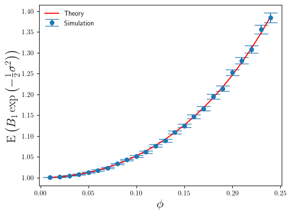
Below in Figure 1 I’ve shown a plot of the expectation of , relative to the true bias correction factor , as a function of . The red line is based on the theoretical calculation in Eq.3, whilst the blue points are simulation estimates,
Figure 1: Plot of theory and simulation estimates of the average relative error made by the parametric bias correction factor, as we increase the variance of the log-normal data.
The agreement between simulation and theory is very good. But even for these small values of we can see the error that makes in estimating the correct bias correction factor is significant – nearly 40% relative error at . For , the value of is 2.24 at . Whilst this is large for the additive log-scale noise, it is not ridiculously large. It shows that the presence of the divergence at is strongly felt even a long way away from that divergence point.
The error bars on the simulation estimates correspond to standard-errors of the mean. In calculating the standard-errors of the mean I’ve used the theoretical calculation of (derived from Eq.5), rather than the simulation sample estimate of it. The reason being that once one goes above about and above , the variance (over different sets of simulation runs) of becomes large itself, and so obtaining a stable accurate simulation estimate of requires such a prohibitively large number of simulations (way greater than 100000) that estimating from a simulation sample becomes impractical. So I used the theoretical result instead. Hence also why the plot below is restricted to .
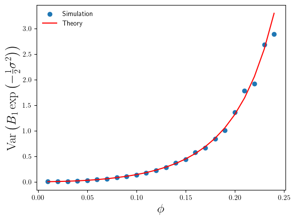
For the range , where the simulation sample size is sufficiently large enough that we can trust our simulation sample based estimates of , we can compare them with the theoretical values. This comparison is plotted in Figure 2 below.
Figure 2: Plot of theory and simulation estimates of the variance of the relative error made by the parametric bias correction factor, as we increase the variance of the log-normal data.
We can see that the simulation estimates of confirm the accuracy of the theoretical result in Eq.5, and consequently confirm the validity of the standard error estimates in Figure 1.
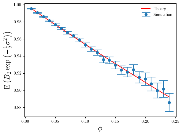
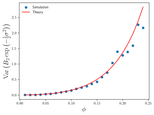
Okay, so that’s confirmed the ‘surprising’ behaviour of the bias-correction estimate , but what about ? How do simulation estimates of and compare to the theoretical results in Eq.4 and Eq.6 ? I’ve plotted these in Figures 3 and 4 below.
Figure 3: Plot of theory and simulation estimates of the average relative error made by the non-parametric bias correction factor, as we increase the variance of the log-normal data.
The accuracy of is much better than that of . By comparison only makes a 10% relative error (under-estimate) on average at , compared to the 40% over-estimate of (on average). We can also see that the magnitude of the relative error increases slowly as increases, again in constrast with the rapid increase in the relative error made by (in Figure 1).
Figure 4: Plot of theory and simulation estimates of the variance of the relative error made by the non-parametric bias correction factor, as we increase the variance of the log-normal data.
Conclusion
So, the theoretical derivations and analysis I did of and turned out to be correct. What did I learn from this? Three things. Firstly, even areas of mathematics that you understand well, have worked with for a long time, and are relatively simple in mathematical terms (e.g. just a univariate distribution) have the capacity to surprise you. Secondly, given this capacity to surprise it is always a good idea to check your mathematical hunches, even with a simple calculation, no matter how confident you are in those hunches. Thirdly, don’t leave it 25 years to check your mathematical hunches. The evaluation of those integrals defining and only took me a couple of minutes. If I had calculated those integrals 25 years ago, I wouldn’t be feeling so stupid now.
Here’s an interesting little coding challenge for you, with a curious data twist at the end. Less of an Advent of Code challenge and more of a Christmas Cracker puzzle.
Without knowing anything about you, I will make a prediction about the size of the files you have on your computer. Christmas magic? Maybe. Read on to find out.
There are two parts to this puzzle
Part 1 – Obtain a list of file sizes (in bytes) of all the files on your computer that are in a high-level directory and its sub-directories. We’re talking here about files with a non-zero file size. We also talking about actual files, so the folders/directories themselves should not be included, just their file contents. If this is your own laptop the high-level directory could be the Documents directory (if on Windows). Obviously, you’ll need to have permission to recurse over all the sub-directories. You should choose a starting directory that has a reasonably large number of files in total across all its sub-directories.
Part 2 – Calculate the proportion of files whose file size starts with a 1. So, if you had 10 files of sizes, 87442, 78922, 3444, 9653, 197643, 26768, 8794787, 22445, 7654, 56573, then the proportion of files whose file size starts with a 1 is 0.1 or 10%.
The overall goal
The goal is to write code that performs the two parts of the challenge in as efficient a way as possible. You can use whatever programming languages you want to perform the two parts – you might use the command line for the first part and a high-level programming language for the second, or you might use a high-level programming language for both parts.
I used Python for both parts and used the Documents directory on my laptop as my starting directory. I had 96351 files in my Documents folder and its sub-directories. The proportion of my files that have a size starting with 1 is approximately 0.31, or 31%.
The twist
Now for the curious part. You should get a similar proportion, that is, around 30%. I will explain why in a separate post (part 2) in the new year, and why if you don’t it can tell us something interesting about the nature of the files on your computer.
You have some prototype Data Science code based on an algorithm you have designed. The code needs to be productionized, and so sped up to meet the specified production run-times. If you stick to your existing technology stack, unless the runtimes of your prototype code are within a factor of 1000 of your target production runtimes, you’ll need a bigger, better algorithm. There is a limit to what speed up your technology stack can achieve. Why is this? Read on and I’ll explain. And I’ll explain what you can do if you need more than a 1000-fold speed up of your prototype.
Speeding up your code with your current tech stack
There are two ways in which you can speed up your prototype code,
Improve the efficiency of the language constructs used, e.g. in Python replacing for loops with list comprehensions or maps, refactoring subsections of the code etc.
Horizontal scaling of your current hardware, e.g. adding more nodes to a compute cluster, adding more executors to the pool in a Spark cluster.
Point 2 assumes that your calculation is compute bound and not memory bound, but we’ll stick with that assumption for this article. We also exclude the possibility that the productionization team can invent or buy a new technology that is sufficiently different or better than your current tech stack – it would be an unfair ask of the ML engineers to have to invent a whole new technology just to compensate for your poor prototype. They may be able to to, but we are talking solely about using your current tech stack and we assume that it does have some capacity to be horizontally scaled.
So what speed ups can we expect from points 1 and 2 above? Point 1 is always possible. There are always opportunities for improving code efficiency that you or another person will spot when looking at the code for a second time. A more experienced programmer reviewing the code can definitely help. But let’s assume that you’re a reasonably experienced Data Scientist yourself. It is unlikely that your code is so bad that a review by someone else would speed it up by more than a factor of 10 or so.
So if the most we expect from code efficiency improvements is a factor 10 speed up, what speed up can we additionally get from horizontal scaling of your existing tech stack? A factor of 100 at most. Where does this limit of 100 come from? Amdahl’s law.
Amdahl’s law
Amdahl’s law is a great little law. Its origins are in High Performance Computing (HPC), but it has a very intuitive basis and so is widely applicable. Because of that it is worth explaining in detail.
Imagine we have a task that currently takes time T to run. Part of that task can be divided up and performed by separate workers or resources such as compute nodes. Let’s use P to denote the fraction of the task that can be divided up. We choose the symbol P because this part of the overall task can be parallelized. The fraction that can’t be divided up we denote by S, because it is the non-parallelizable or serial part of the task. The serial part of the task represents things like unavoidable overhead and operations in manipulating input and output data-structures and so on.
Obviously, since we’re talking about fractions of the overall runtime T, the fractions P and S must sum to 1, i.e.
The parallelizable part of the task takes time TP to run, whilst the serial part takes time TS to run.
What happens if we do parallelize that parallelizable component P? We’ll parallelize it using N workers or executors. When N=1, the parallelizable part took time TP to run, so with N workers it should (in an ideal world) take time TP/N to run. Now our overall run time, as a function of N is,
This is Amdahl’s law1. It looks simple but let’s unpack it in more detail. We can write the speed up factor in going from T(N=1) to T(N) as,
The figure below shows plots of the speed-up factor against N, for different values of S.
From the plot in the figure, you can see that the speed up factor initially looks close to linear in N and then saturates. The speed up at saturation depends on the size of the serial component S. There is clearly a limit to the amount of speed up we can achieve. When N is large, we can approximate the speed up factor in Eq.3 as,
From Eq.4 (or from Eq.3) we can see the limiting speed up factor is 1/S. The mathematical approximation in Eq.4 hides the intuition behind the result. The intuition is this; if the total runtime is,
then at some point we will have made N big enough that P/N is smaller than S. This means we have reduced the runtime of the parallelizable part to below that of the serial part. The largest contribution to the overall runtime is now the serial part, not the parallelizable part. Increasing N further won’t change this. We have hit a point of rapidly diminishing returns. And by definition we can’t reduce S by any horizontal scaling. This means that when P/N becomes comparable to S, there is little point in increasing N further and we have effectively reached the saturation speed up.
How small is S?
This is the million-dollar question, as the size of S determines the limiting speed up factor we can achieve through horizontal scaling. A larger value of S means a smaller speed up factor limit. And here’s the depressing part – you’ll be very lucky to get S close to 1%, which would give you a speed up factor limit of 100.
A real-world example
To explain why S = 0.01 is around the lowest serial fraction you’ll observe in a real calculation, I’ll give you a real example. I first came across Amdahl’s law in 2007/2008, whilst working on a genomics project, processing very high-dimensional data sets2. The calculations I was doing were statistical hypothesis tests run multiple times.
This is an example of an “embarrassingly parallel” calculation since it just involves splitting up a dataframe into subsets of rows and sending the subsets to the worker nodes of the cluster. There is no sophistication to how the calculation is parallelized, it is almost embarrassing to do – hence the term “embarrassingly parallel”.
The dataframe I had was already sorted in the appropriate order, so parallelization consisted of taking a small number of rows off the top of dataframe and sending to a worker node and repeating. Mathematically, on paper, we had S=0. Timings of actual calculations with different numbers of compute nodes and fitting an Amdahl’s law curve to those timings revealed we had something between S=0.01 and S=0.05.
A value of S=0.01 gaves us a maximum speed up factor of 100 from horizontal scaling. And this was for a problem that on paper had S=0. In reality, there is always some code overhead in manipulating the data. A more realistic limit on S for an average complexity piece of Data Science code would be S=0.05 or S=0.1, meaning we should expect limits on the speed up factor of between 10 and 20.
What to do?
Disappointing isn’t it!? Horizontal scaling will speed up our calculation by at most a factor of 100, and more likely only a factor of 10-20. What does it mean for productionizing our prototype code? If we also include the improvements in the code efficiency, the most we’re likely to be able to speed up our prototype code by is a factor of 1000 overall. It means that as a Data Scientist you have a responsibility to ensure the runtime of your initial prototype is within a factor of 1000 of the production runtime requirements.
If a speed up of 1000 isn’t enough to hit the production run-time requirements, what can we do? Don’t despair. You have several options. Firstly, you can always change the technology underpinning your tech stack. Despite what I said at the beginning of this post, if you are repeatedly finding that horizontal scaling of your current tech stack does not give you the speed-up you require, then there may be a case for either vertical scaling the runtime performance of each worker node or using a superior tech stack if one exists.
If improvement by vertical scaling of individual compute nodes is not possible, then there are still things you can do to mitigate the situation. Put the coffee on, sharpen your pencil, and start work on designing a faster algorithm. There are two approaches you can use here,
Reduce the performance requirements: This could be lowering the accuracy through approximations that are simpler and quicker to calculate. For example, if your code involves significant matrix inversion operations you may be able to approximate a matrix by its diagonal and explicitly hard code the calculation of its inverse rather than performing expensive numerical inversion of the full matrix.
Construct a better algorithm: There are no easy recipes here. You can get some hints on where to focus your effort and attention by identifying the runtime bottlenecks in your initial prototype. This can be done using code profiling tools. Once a bottleneck has been identified, you can then progress by simplifying the problem and constructing a toy problem that has the same mathematical characteristics as the original bottleneck. By speeding up the toy problem you will learn a lot. You can then apply those learnings, even if only approximately, to the original bottleneck problem.
When I first stumbled across Amdahl’s law, I mentioned it to a colleague working on the same project as I was. They were a full-stack software developer and immediately, said “oh, you mean Amdahl’s law about limits on the speed you can write to disk?”. It turns out there is another Amdahl’s Law, often called “Amdahl’s Second Law”, or “Amdahl’s Other Law”, or “Amdahl’s Lesser Law”, or “Amdahl’s Rule-Of-Thumb”. See this blog post, for example, for more details on Amdahl’s Second Law.
The bisection algorithm is a very simple algorithm for finding the root of a 1-D function.
Working out the number of iterations of the algorithm required to determine the root location within a specified tolerance can be determined from a very simple little hack, which I explain here.
Things get more interesting when we consider variants of the bisection algorithm, where we cut an interval into unequal portions.
</TL;DR>
A little while ago a colleague mentioned that they were repeatedly using an off-the-shelf bisection algorithm to find the root of a function. The algorithm required the user to specify the number of iterations to run the bisection for. Since my colleague was running the algorithm repeatedly they wanted to set the number of iterations efficiently and also to achieve a guaranteed level of accuracy, but they didn’t know how to do this.
I mentioned that it was very simple to do this and it was a couple of lines of arithmetic in a little hack that I’d used many times. Then I realised that the hack was obvious and known to me because I was old – I’d been doing this sort of thing for years. My colleague hadn’t. So I thought the hack would be a good subject for a short blog post.
The idea behind a bisection algorithm is simple and illustrated in Figure 1 below.
Figure 1: Schematic of how the bisection algorithm works
At each iteration we determine whether the root is to the right of the current mid-point, in the right-hand interval, or to the left of the current mid-point, in the left-hand interval. In either case, the range within which we locate the root halves. We have gone from knowing it was in the interval , which has width , to knowing it is in an interval of width . So with every iteration we reduce our uncertainty of where the root is located by half. After iterations we have reduced our initial uncertainty by . Given our initial uncertainty is determined by the initial bracketing of the root, i.e. an interval of width , we can now work out that after iterations we have narrowed down the root to an interval of width . Now if we want to locate the root to within a tolerance , we just have to keep iterating until the uncertainty reaches . That is, we run for iterations where satisfies,
Strictly speaking we need to run for iterations. Usually I will add on a few extra iterations, e.g. 3 to 5, as an engineering safety factor.
As a means of easily and quickly determining the number of iterations to run a bisection algorithm the calculation above is simple, easy to understand and a great little hack to remember.
Is bisection optimal?
The bisection algorithm works by dividing into two our current estimate of the interval in which the root lies. Dividing the interval in two is efficient. It is like we are playing the childhood game “Guess Who”, where we ask questions about the characters’ features in order to eliminate them.
Asking about a feature that approximately half the remaining characters possess is the most efficient – it has a reasonable probability of applying to the target character and eliminates half of the remaining characters. If we have single question, with a binary outcome and a probability of one of those outcomes, then the question that has maximizes the expected information (the entropy), .
Dividing the interval unequally
When we first played “Guess Who” as kids we learnt that asking questions with a much lower probability of being correct didn’t win the game. Is the same true for our root finding algorithm? If instead we divide each interval into unequal portions is the root finding less efficient than when we bisect the interval?
Let’s repeat the derivation but with a different cut-point e.g. 25% along the current interval bracketing the root. In general we can test whether the root is to the left of right of a point that is a proportion along the current interval, meaning the cut-point is . At each iteration we don’t know in advance which side of the cut-point the root lies until we test for it, so in trying to determine in advance the number of iterations we need to run, we have to assume the worst case scenario and assume that the root is still in the larger of the two intervals. The reduction in uncertainty is then, . Repeating the derivation we find that we have to run at least,
iterations to be guaranteed that we have located the root to within .
Now to determine the cut-point that minimizes the upper bound on number of iterations required, we simply differentiate the expression above with respect to . Doing so we find,
and
The minimum of is at , although is not a stationary point of the upper bound , as has a discontinuous gradient there.
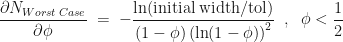
That is the behaviour of the worst-case scenario. A similar analysis can be applied to the best-case scenario – we simply replace with in all the above formula. That is, in the best-case scenario the number of iterations required is given by,
Here, the maximum of the best-case number of iterations occurs when .
That’s the worst-case and best-case scenarios, but how many iterations do we expect to use on average? Let’s look at the expected reduction in uncertainty in the root location after iterations. In a single iteration a root that is randomly located within our interval will lie, with probability , in segement to the left of our cut-point and leads to a reduction in the uncertainty by a factor of . Similarly, we get a reduction in uncertainty of with probability if our randomly located root is to the right of the cut-point. So after iterations the expected reduction in uncertainty is,
Using this as an approximation to determine the typical number of iterations, we get,
This still isn’t the expected number of iterations, but to see how it compares Figure 2 belows shows simulation estimates of plotted against when the root is random and uniformly distributed within the original interval.
Number of iterations required for the different root finding methods.
For Figure 2 we have set . Also plotted in Figure 2 are our three theoretical estimates, . The stepped structure in these 3 integer quantities is clearly apparent, as is how many more iterations are required under the worst case method when .
The expected number of iterations required, , actually shows a rich structure that isn’t clear unless you zoom in. Some aspects of that structure were unexpected, but requires some more involved mathematics to understand. I may save that for a follow-up post at a later date.
I have recently needed to do some work evaluating high-order derivatives of composite functions. Namely, given a function , evaluate the derivative of the composite function . That is, we define to be the function obtained by iterating the base function times. One approach is to make recursive use of the Faa di Bruno formula,
Eq.(1)
The fact that the exponential partial Bell polynomials are available within the symbolic algebra Python package, makes this initially an attractive route to evaluating the required derivatives. In particular, I am interested in evaluating the derivatives at and I am focusing on odd functions of , for which is then obviously a fixed-point. This means I only have to supply numerical values for the derivatives of my base function evaluated at , rather than supplying a function that evaluates derivatives of at any point .
Given the Taylor expansion of about we can easily write code to implement the Faa di Bruno formula using sympy. A simple bit of pseudo-code to represent an implementation might look like,
Generate symbols.
Generate and store partial Bell polynomials up to known required order using the symbols from step 1.
Initialize coefficients of Taylor expansion of the base function.
Substitute numerical values of derivatives from previous iteration into symbolic representation of polynomial.
Sum required terms to get numerical values of all derivatives of current iteration.
Repeat steps 4 & 5.
I show python code snippets below implementing the idea. First we generate and cache the Bell polynomials,
 # generate and cache Bell polynomials
 bellPolynomials = {}
 for n in range(1, nMax+1):
      for k in range(1, n+1):
         bp_tmp = sympy.bell(n, k, symbols_tmp)
         bellPolynomials[str(n) + '_' + str(k)] = bp_tmp
Then we iterate over the levels of function composition, substituting the numerical values of the derivatives of the base function into the Bell polynomials,
for iteration in range(nIterations):
    if( verbose ):
        print( "Evaluating derivatives for function iteration " + str(iteration+1) )

    for n in range(1, nMax+1):
        sum_tmp = 0.0
        for k in range(1, n+1):
            # retrieve kth derivative of base function at previous iteration
            f_k_tmp = derivatives_atFixedPoint_tmp[0, k-1]

            #evaluate arguments of Bell polynomials
            bellPolynomials_key = str( n ) + '_' + str( k )
            bp_tmp = bellPolynomials[bellPolynomials_key]
            replacements = [( symbols_tmp[i],
            derivatives_atFixedPoint_tmp[iteration, i] ) for i in range(n-k+1) ]
            sum_tmp = sum_tmp + ( f_k_tmp * bp_tmp.subs(replacements) )

        derivatives_atFixedPoint_tmp[iteration+1, n-1] = sum_tmp
Okay – this isn’t really making use true recursion, merely looping, but the principle is the same. The problem one encounters is that the manipulation of the symbolic representation of the polynomials is slow, and run-times slow significantly for .
However, the derivative can alternatively be expressed as a sum over partitions of n as,
Eq.(2)
where the sum is taken over all non-negative integers tuples that satisfy . That is, the sum is taken over all partitions of n. Fairly obviously the Faa di Bruno formula is just a re-arrangement of the above equation, made by collecting terms involving together, and as such that rearrangement gives the fundamental definition of the partial Bell polynomial.
I’d shied away from the more fundamental form of Eq.(2) in favour of Eq.(1) as I believed the fact that a number of terms had already been collected together in the form of the Bell polynomial would make any implementation that used them quicker. However, the advantage of the form in Eq.(2) is that the summation can be entirely numeric, provided an efficient generator of partitions of n is available to us. Fortunately, sympy also contains a method for iterating over partitions. Below are code snippets that implement the evaluation of using Eq.(2). First we generate and store the partitions,
# store partitions
pStore = {}
for k in range( n ):
    # get partition iterator
    pIterator = partitions(k+1)
    pStore[k] = [p.copy() for p in pIterator]
After initializing arrays to hold the derivatives of the current function iteration we then loop over each iteration, retrieving each partition and evaluating the product in the summand of Eq.(2). Obviously, it is relatively easy working on the log scale, as shown in the code snippet below,
# loop over function iterations
for iteration in range( nIterations ):

    if( verbose==True ):
        print( "Evaluating derivatives for function iteration " + str(iteration+1)  )

    for k in range( n ):
        faaSumLog = float( '-Inf' )
        faaSumSign = 1

        # get partitions
        partitionsK = pStore[k]
        for pidx in range( len(partitionsK) ):
            p = partitionsK[pidx]
            sumTmp = 0.0
            sumMultiplicty = 0
            parityTmp = 1
            for i in p.keys():
                value = float(i)
                multiplicity = float( p[i] )
                sumMultiplicty += p[i]
                sumTmp += multiplicity * currentDerivativesLog[i-1]
                sumTmp -= gammaln( multiplicity + 1.0 )
                sumTmp -= multiplicity * gammaln( value + 1.0 )
                parityTmp *= np.power( currentDerivativesSign[i-1], multiplicity )

            sumTmp += baseDerivativesLog[sumMultiplicty-1]
            parityTmp *= baseDerivativesSign[sumMultiplicty-1]

            # now update faaSum on log scale
            if( sumTmp > float( '-Inf' ) ):
                if( faaSumLog > float( '-Inf' ) ):
                    diffLog = sumTmp - faaSumLog
                    if( np.abs(diffLog) = 0.0 ):
                            faaSumLog = sumTmp
                            faaSumLog += np.log( 1.0 + (float(parityTmp*faaSumSign) * np.exp( -diffLog )) )
                            faaSumSign = parityTmp
                        else:
                            faaSumLog += np.log( 1.0 + (float(parityTmp*faaSumSign) * np.exp( diffLog )) )
                    else:
                        if( diffLog > thresholdForExp ):
                            faaSumLog = sumTmp
                            faaSumSign = parityTmp
                else:
                    faaSumLog = sumTmp
                    faaSumSign = parityTmp

        nextDerivativesLog[k] = faaSumLog + gammaln( float(k+2) )
        nextDerivativesSign[k] = faaSumSign
Now let’s run both implementations, evaluating up to the 15th derivative for 4 function iterations. Here my base function is . A plot of the base function is shown below in Figure 1.
Figure 1: Plot of the base function
The base function has a relatively straight forward Taylor expansion about ,
Eq.(3)
and so supplying the derivatives, , of the base function is easy. The screenshot below shows a comparison of for . As you can see we obtain identical output whether we use sympy’s Bell polynomials or sympy’s partition iterator.
The comparison of the implementations is not really a fair one. One implementation is generating a lot of symbolic representations that aren’t really needed, whilst the other is keeping to entirely numeric operations. However, it did highlight several points to me,
Directly working with partitions, even up to moderate values of , e.g. , can be tractable using the sympy package in python.
Sometimes the implementation of the more concisely expressed representation (in this case in terms of Bell polynomials) can lead to an implementation with significantly longer run-times, even if the more concise representation can be implemented concisely (less lines of code).
I’ve put the code for both methods of evaluating the derivatives of an iterated function as a gist on github.
At the moment the functions take an array of Taylor expansion coefficients, i.e. they assume the point at which derivatives are requested is a fixed point of the base function. At some point I will add methods that take a user-supplied function for evaluating the derivative, , of the base function at any point t and will return the derivatives, of the iterated function.
I haven’t yet explored whether, for reasonable values of n (say ), I need to work on the log scale, or whether direct evaluation of the summand will be sufficiently accurate and not result in overflow error.


![\mathbb{E}\left ( B_{1}\right )\;=\; \left( 2\pi\sigma^{2}\right)^{-\frac{N}{2}}\int_{{\mathbb{R}}^{N}} d{\underline{x}}\exp\left [-\frac{1}{2\sigma^{2}}\left ( \underline{x} - \mu\underline{1}_{N}\right )^{\top}\left ( \underline{x} - \mu\underline{1}_{N}\right )\right ] \exp\left[ \frac{1}{2} \underline{x}^{\top}\underline{\underline{M}}\underline{x}\right ]](https://s0.wp.com/latex.php?latex=%5Cmathbb%7BE%7D%5Cleft+%28+B_%7B1%7D%5Cright+%29%5C%3B%3D%5C%3B+%5Cleft%28+2%5Cpi%5Csigma%5E%7B2%7D%5Cright%29%5E%7B-%5Cfrac%7BN%7D%7B2%7D%7D%5Cint_%7B%7B%5Cmathbb%7BR%7D%7D%5E%7BN%7D%7D+d%7B%5Cunderline%7Bx%7D%7D%5Cexp%5Cleft+%5B-%5Cfrac%7B1%7D%7B2%5Csigma%5E%7B2%7D%7D%5Cleft+%28+%5Cunderline%7Bx%7D+-+%5Cmu%5Cunderline%7B1%7D_%7BN%7D%5Cright+%29%5E%7B%5Ctop%7D%5Cleft+%28+%5Cunderline%7Bx%7D+-+%5Cmu%5Cunderline%7B1%7D_%7BN%7D%5Cright+%29%5Cright+%5D+%5Cexp%5Cleft%5B+%5Cfrac%7B1%7D%7B2%7D+%5Cunderline%7Bx%7D%5E%7B%5Ctop%7D%5Cunderline%7B%5Cunderline%7BM%7D%7D%5Cunderline%7Bx%7D%5Cright+%5D&bg=ffffff&fg=111111&s=0&c=20201002)


![\mathbb{E}\left ( B_{2}\right )\;=\;\frac{1}{N}\sum_{i=1}^{N} \left( 2\pi\sigma^{2}\right)^{-\frac{N}{2}}\int_{{\mathbb{R}}^{N}} d{\underline{x}}\exp\left [-\frac{1}{2\sigma^{2}}\left ( \underline{x} - \mu\underline{1}_{N}\right )^{\top}\left ( \underline{x} - \mu\underline{1}_{N}\right )\right ] \exp \left [ \sum_{j=1}^{N}\left ( \delta_{ij} - \frac{1}{N}\right )x_{j}\right ]](https://s0.wp.com/latex.php?latex=%5Cmathbb%7BE%7D%5Cleft+%28+B_%7B2%7D%5Cright+%29%5C%3B%3D%5C%3B%5Cfrac%7B1%7D%7BN%7D%5Csum_%7Bi%3D1%7D%5E%7BN%7D+%5Cleft%28+2%5Cpi%5Csigma%5E%7B2%7D%5Cright%29%5E%7B-%5Cfrac%7BN%7D%7B2%7D%7D%5Cint_%7B%7B%5Cmathbb%7BR%7D%7D%5E%7BN%7D%7D+d%7B%5Cunderline%7Bx%7D%7D%5Cexp%5Cleft+%5B-%5Cfrac%7B1%7D%7B2%5Csigma%5E%7B2%7D%7D%5Cleft+%28+%5Cunderline%7Bx%7D+-+%5Cmu%5Cunderline%7B1%7D_%7BN%7D%5Cright+%29%5E%7B%5Ctop%7D%5Cleft+%28+%5Cunderline%7Bx%7D+-+%5Cmu%5Cunderline%7B1%7D_%7BN%7D%5Cright+%29%5Cright+%5D%C2%A0+%5Cexp+%5Cleft+%5B+%5Csum_%7Bj%3D1%7D%5E%7BN%7D%5Cleft+%28+%5Cdelta_%7Bij%7D+-+%5Cfrac%7B1%7D%7BN%7D%5Cright+%29x_%7Bj%7D%5Cright+%5D&bg=ffffff&fg=111111&s=0&c=20201002)

![\mathbb{E}\left ( B_{2}\right )\;=\; \exp \left [ \frac{\sigma^{2}}{2}\left ( 1\;-\;\frac{1}{N}\right )\right ]](https://s0.wp.com/latex.php?latex=%5Cmathbb%7BE%7D%5Cleft+%28+B_%7B2%7D%5Cright+%29%5C%3B%3D%5C%3B+%5Cexp+%5Cleft+%5B+%5Cfrac%7B%5Csigma%5E%7B2%7D%7D%7B2%7D%5Cleft+%28+1%5C%3B-%5C%3B%5Cfrac%7B1%7D%7BN%7D%5Cright+%29%5Cright+%5D&bg=ffffff&fg=111111&s=0&c=20201002)


![{\rm Var}\left ( B_{2}\right)\;=\; \left ( 1 - \frac{1}{N}\right )\exp \left [ \sigma^{2}\left ( 1 - \frac{2}{N}\right )\right ]\;+\;\frac{1}{N}\exp \left [ 2\sigma^{2}\left ( 1 - \frac{1}{N}\right )\right ]\;-\; \exp \left [ \sigma^{2}\left ( 1 - \frac{1}{N}\right )\right ]](https://s0.wp.com/latex.php?latex=%7B%5Crm+Var%7D%5Cleft+%28+B_%7B2%7D%5Cright%29%5C%3B%3D%5C%3B+%5Cleft+%28+1+-+%5Cfrac%7B1%7D%7BN%7D%5Cright+%29%5Cexp+%5Cleft+%5B+%5Csigma%5E%7B2%7D%5Cleft+%28+1+-+%5Cfrac%7B2%7D%7BN%7D%5Cright+%29%5Cright+%5D%5C%3B%2B%5C%3B%5Cfrac%7B1%7D%7BN%7D%5Cexp+%5Cleft+%5B+2%5Csigma%5E%7B2%7D%5Cleft+%28+1+-+%5Cfrac%7B1%7D%7BN%7D%5Cright+%29%5Cright+%5D%5C%3B-%5C%3B+%5Cexp+%5Cleft+%5B+%5Csigma%5E%7B2%7D%5Cleft+%28+1+-+%5Cfrac%7B1%7D%7BN%7D%5Cright+%29%5Cright+%5D&bg=ffffff&fg=111111&s=0&c=20201002)


![[x_{lower}, x_{upper}]](https://s0.wp.com/latex.php?latex=%5Bx_%7Blower%7D%2C+x_%7Bupper%7D%5D&bg=ffffff&fg=111111&s=0&c=20201002) , which has width
, which has width  , to knowing it is in an interval of width
  . So with every iteration we reduce our uncertainty of where the root is located by half. After
  . Given our initial uncertainty is determined by the initial bracketing of the root, i.e. an interval of width
  , we can now work out that after
  . Now if we want to locate the root to within a tolerance
  , we just have to keep iterating until the uncertainty reaches
 iterations. Usually I will add on a few extra iterations, e.g. 3 to 5, as an engineering safety factor.
 of one of those outcomes, then the question that has
  maximizes the expected information (the entropy),
  .
. . At each iteration we don’t know in advance which side of the cut-point the root lies until we test for it, so in trying to determine in advance the number of iterations we need to run, we have to assume the worst case scenario and assume that the root is still in the larger of the two intervals. The reduction in uncertainty is then,
 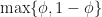 . Repeating the derivation we find that we have to run at least,
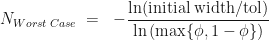
 .
.

 is at
is at  , although
  is not a stationary point of the upper bound
  with
with  in all the above formula. That is, in the best-case scenario the number of iterations required is given by,
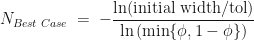
 .
.  with probability
 plotted against
 . Also plotted in Figure 2 are our three theoretical estimates,
  . The stepped structure in these 3 integer quantities is clearly apparent, as is how many more iterations are required under the worst case method when
  .
. , actually shows a rich structure that isn’t clear unless you zoom in. Some aspects of that structure were unexpected, but requires some more involved mathematics to understand. I may save that for a follow-up post at a later date.
 , evaluate the
  derivative of the composite function
  . That is, we define
  to be the function obtained by iterating the base function
 times. One approach is to make recursive use of the
  Eq.(1)
 are available within the
  symbolic algebra Python package, makes this initially an attractive route to evaluating the required derivatives. In particular, I am interested in evaluating the derivatives at
  and I am focusing on odd functions of
  , for which
  .
. Eq.(2)
 that satisfy
  . That is, the sum is taken over all partitions of n. Fairly obviously the Faa di Bruno formula is just a re-arrangement of the above equation, made by collecting terms involving
  together, and as such that rearrangement gives the fundamental definition of the partial Bell polynomial.
 using Eq.(2). First we generate and store the partitions,
 . A plot of the base function is shown below in Figure 1.
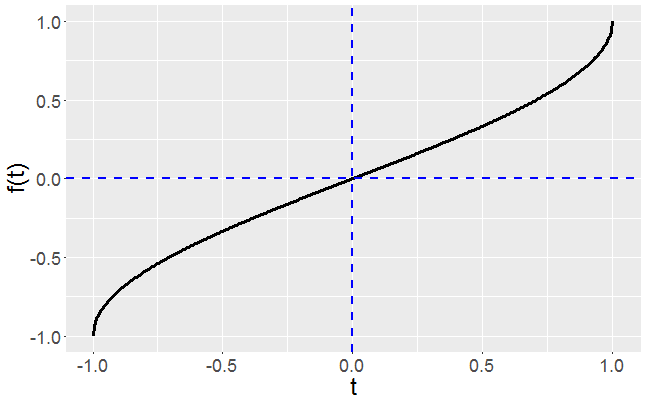

 Eq.(3)
 , of the base function is easy. The screenshot below shows a comparison of
  for
for  . As you can see we obtain identical output whether we use sympy’s Bell polynomials or sympy’s partition iterator.
 , e.g.
  , can be tractable using the sympy package in python.
 derivative,
  , of the base function at any point t and will return the derivatives,
  of the iterated function.
 ), I need to work on the log scale, or whether direct evaluation of the summand will be sufficiently accurate and not result in overflow error.