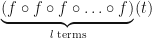
I have recently needed to do some work evaluating high-order derivatives of composite functions. Namely, given a function , evaluate the derivative of the composite function . That is, we define to be the function obtained by iterating the base function times. One approach is to make recursive use of the Faa di Bruno formula,

     Eq.(1)

The fact that the exponential partial Bell polynomials 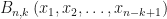are available within the symbolic algebra Python package, makes this initially an attractive route to evaluating the required derivatives. In particular, I am interested in evaluating the derivatives at and I am focusing on odd functions of , for which is then obviously a fixed-point. This means I only have to supply numerical values for the derivatives of my base function evaluated at , rather than supplying a function that evaluates derivatives of at any point .

Given the Taylor expansion of about we can easily write code to implement the Faa di Bruno formula using sympy. A simple bit of pseudo-code to represent an implementation might look like,

1. Generate symbols.
2. Generate and store partial Bell polynomials up to known required order using the symbols from step 1.
3. Initialize coefficients of Taylor expansion of the base function.
4. Substitute numerical values of derivatives from previous iteration into symbolic representation of polynomial.
5. Sum required terms to get numerical values of all derivatives of current iteration.
6. Repeat steps 4 & 5.

I show python code snippets below implementing the idea. First we generate and cache the Bell polynomials,

 # generate and cache Bell polynomials
 bellPolynomials = {}
 for n in range(1, nMax+1):
      for k in range(1, n+1):
         bp_tmp = sympy.bell(n, k, symbols_tmp)
         bellPolynomials[str(n) + '_' + str(k)] = bp_tmp

Then we iterate over the levels of function composition, substituting the numerical values of the derivatives of the base function into the Bell polynomials,

for iteration in range(nIterations):
    if( verbose ):
        print( "Evaluating derivatives for function iteration " + str(iteration+1) )

    for n in range(1, nMax+1):
        sum_tmp = 0.0
        for k in range(1, n+1):
            # retrieve kth derivative of base function at previous iteration
            f_k_tmp = derivatives_atFixedPoint_tmp[0, k-1]

            #evaluate arguments of Bell polynomials
            bellPolynomials_key = str( n ) + '_' + str( k )
            bp_tmp = bellPolynomials[bellPolynomials_key]
            replacements = [( symbols_tmp[i],
            derivatives_atFixedPoint_tmp[iteration, i] ) for i in range(n-k+1) ]
            sum_tmp = sum_tmp + ( f_k_tmp * bp_tmp.subs(replacements) )

        derivatives_atFixedPoint_tmp[iteration+1, n-1] = sum_tmp

Okay – this isn’t really making use true recursion, merely looping, but the principle is the same. The problem one encounters is that the manipulation of the symbolic representation of the polynomials is slow, and run-times slow significantly for .

However, the derivative can alternatively be expressed as a sum over partitions of n as,

  Eq.(2)

where the sum is taken over all non-negative integers tuples that satisfy . That is, the sum is taken over all partitions of  n. Fairly obviously the Faa di Bruno formula is just a re-arrangement of the above equation, made by collecting terms involving together, and as such that rearrangement gives the fundamental definition of the partial Bell polynomial.

I’d shied away from the more fundamental form of Eq.(2) in favour of Eq.(1) as I believed the fact that a number of terms had already been collected together in the form of the Bell polynomial would make any implementation that used them quicker. However, the advantage of the form in Eq.(2) is that the summation can be entirely numeric, provided an efficient generator of partitions of n is available to us. Fortunately, sympy also contains a method for iterating over partitions. Below are code snippets that implement the evaluation of using Eq.(2). First we generate and store the partitions,

# store partitions
pStore = {}
for k in range( n ):
    # get partition iterator
    pIterator = partitions(k+1)
    pStore[k] = [p.copy() for p in pIterator]

After initializing arrays to hold the derivatives of the current function iteration we then loop over each iteration, retrieving each partition and evaluating the product in the summand of Eq.(2). Obviously, it is relatively easy working on the log scale, as shown in the code snippet below,

# loop over function iterations
for iteration in range( nIterations ):

    if( verbose==True ):
        print( "Evaluating derivatives for function iteration " + str(iteration+1)  )

    for k in range( n ):
        faaSumLog = float( '-Inf' )
        faaSumSign = 1

        # get partitions
        partitionsK = pStore[k]
        for pidx in range( len(partitionsK) ):
            p = partitionsK[pidx]
            sumTmp = 0.0
            sumMultiplicty = 0
            parityTmp = 1
            for i in p.keys():
                value = float(i)
                multiplicity = float( p[i] )
                sumMultiplicty += p[i]
                sumTmp += multiplicity * currentDerivativesLog[i-1]
                sumTmp -= gammaln( multiplicity + 1.0 )
                sumTmp -= multiplicity * gammaln( value + 1.0 )
                parityTmp *= np.power( currentDerivativesSign[i-1], multiplicity )	

            sumTmp += baseDerivativesLog[sumMultiplicty-1]
            parityTmp *= baseDerivativesSign[sumMultiplicty-1]

            # now update faaSum on log scale
            if( sumTmp > float( '-Inf' ) ):
                if( faaSumLog > float( '-Inf' ) ):
                    diffLog = sumTmp - faaSumLog
                    if( np.abs(diffLog) = 0.0 ):
                            faaSumLog = sumTmp
                            faaSumLog += np.log( 1.0 + (float(parityTmp*faaSumSign) * np.exp( -diffLog )) )
                            faaSumSign = parityTmp
                        else:
                            faaSumLog += np.log( 1.0 + (float(parityTmp*faaSumSign) * np.exp( diffLog )) )
                    else:
                        if( diffLog > thresholdForExp ):
                            faaSumLog = sumTmp
                            faaSumSign = parityTmp
                else:
                    faaSumLog = sumTmp
                    faaSumSign = parityTmp

        nextDerivativesLog[k] = faaSumLog + gammaln( float(k+2) )
        nextDerivativesSign[k] = faaSumSign

Now let’s run both implementations, evaluating up to the 15th derivative for 4 function iterations. Here my base function is . A plot of the base function is shown below in Figure 1.

The base function has a relatively straight forward Taylor expansion about ,

   Eq.(3)

and so supplying the derivatives, , of the base function is easy. The screenshot below shows a comparison of for . As you can see we obtain identical output whether we use sympy’s Bell polynomials or sympy’s partition iterator.

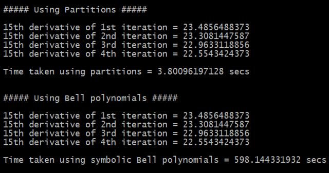
The comparison of the implementations is not really a fair one. One implementation is generating a lot of symbolic representations that aren’t really needed, whilst the other is keeping to entirely numeric operations. However, it did highlight several points to me,

• Directly working with partitions, even up to moderate values of , e.g. , can be tractable using the sympy package in python.
• Sometimes the implementation of the more concisely expressed representation (in this case in terms of Bell polynomials) can lead to an implementation with significantly longer run-times, even if the more concise representation can be implemented concisely (less lines of code).
• The history of the Faa di Bruno formula, and the various associated polynomials and equivalent formalisms (such as the Jabotinksy matrix formalism) is a fascinating one.

I’ve put the code for both methods of evaluating the derivatives of an iterated function as a gist on github.

At the moment the functions take an array of Taylor expansion coefficients, i.e. they assume the point at which derivatives are requested is a fixed point of the base function. At some point I will add methods that take a user-supplied function for evaluating the derivative, , of the base function at any point t and will return the derivatives, of the iterated function.

I haven’t yet explored whether, for reasonable values of n (say ), I need to work on the log scale, or whether direct evaluation of the summand will be sufficiently accurate and not result in overflow error.