Always confirm your mathematical intuition with an explicit calculation, no matter how simple the calculation.
Always confirm your mathematical intuition with an explicit calculation, no matter how well you know the particular area of mathematics.
Don’t leave it 25 years to check your mathematical intuition with a calculation, no matter how confident you are in that intuition.
Introduction
One of the things about mathematics is that it’s not afraid to slap you in the face and stand there laughing at you. Metaphorically speaking, I mean. Mathematics has an infinite capacity to surprise even in areas where you think you can’t be surprised. And you end up looking or feeling like an idiot, with mathematics laughing at you.
This is a salutary lesson about how I thought I understood an area of statistics, but didn’t. The area in question is the log-normal distribution. This is a distribution I first encountered 25 years ago and have worked with almost continuously since.
The problem which slapped me in the face
The particular aspect of the log-normal distribution in question, was what happens when you go from models or estimates on the log-scale, to models or estimates on the ‘normal’ or exponentiated scale. For a log-normal random variable with being the variance of , we have the well-known result,
This is an example of Jensen’s inequality at work. If you apply a non-linear function to a random variable , then the average of the function is not equal to the function of the average. That is, .
In the case of the log-normal distribution, the first equation above tells us that we can relate the to via a simple bias-correction factor . So, if we had a sample of observations of we could estimate the expectation of from an estimate of the expectation of by multiplying by a bias correction factor of . We can estimate from the residuals of our estimate of the expectation of . In this case, I’m going to assume our model is just an estimation of the mean, , which I’ll denote by , and I’m not going to try to decompose any further. If our estimate of is just the sample mean of , then our estimate of would simply be the sample variance, . If we denote our observations by then is given by the formula,
Note the usual Bessel correction that I’ve applied in the calculation of .
We can see from this discussion that the bias correction in going from the log-scale to the ‘normal’ scale is multiplicative in this case. The bias correction factor is given by,
If we had suspected that any bias correction needs to be multiplicative, which seems reasonable given we are going from a log-scale to a normal-scale, then we could easily have estimated a bias correction factor as simply the ratio of the mean of the observations on the normal scale to the exponential of the mean of the observations on the log scale. That is, we can construct a second estimate, , of the bias correction factor needed, with given by,
I tend to refer to the method as a non-parametric method because it is how you would estimate from an estimate of and you only knew the bias correction needed was multiplicative. You wouldn’t explicitly need to make any assumptions about the distribution of the data. In contrast, is specific to the data coming from a log-normal distribution, so I call it a parametric estimate. For these reasons, I tend to prefer using the way of estimating any necessary bias correction factor, as obviously any real data won’t be perfectly log-normal and so the estimator will be more robust whilst also being very simple to calculate.
A colleague asks an awkward question
So far everything I’ve described is well known and pretty standard. However, a few months ago a colleague asked me if there would be any differences between the estimates and ? “Of course”, I said, if the data is not log-normal. “No”, my colleague said. They meant, even if the data was log-normal would there be any differences between the estimates and . Understanding the size of any differences when the parametric assumptions are met would help understand how big the differences could be when the parametric assumptions are violated. “Yeah, there will obviously still be differences between and even if we do have log-normal data, because of sampling variation affecting the two formulae differently. But, I would expect those differences to be small even for moderate sample sizes”, I confidently replied.
I’ve been using those formulae for and for over 25 years and never considered the question my colleague asked. I’d never confirmed my intuition. So 25 years later, I thought I’d do a quick calculation to confirm my intuition. My intuition was very very wrong! I thought it would be interesting to explain the calculations I did and what, to me, was the surprising behaviour of . Note, with hindsight the behaviour I uncovered shouldn’t have been surprising. It was obvious once I’d begun to think about it. It was just that I’d left thinking about it till 25 years too late.
The mathematical detail
The question my colleague was asking was this. If we have i.i.d. observations drawn from a log-normal distribution, i.e.,
what are the expectation values of the bias correction factors and at any finite value of . Do and converge to as , and if so how fast?
Since the are Gaussian random variables we can express these expectation values in terms of simple integrals and we get,
Eq.1
where the matrix is given by,
.
Here is an N-dimensional vector consisting of all ones, and is the identity matrix.
We can similarly express the expectation of and we get,
Eq.2
The matrices in the exponents of the integrands of Eq.1 and Eq.2 are easily diagonalized analytically and so the integrals are relatively easy to evaluate analytically. From this we find,
Eq.3
Eq.4
We can see that as both expressions for the bias correction tend to the correct value of . However, what is noticeable is at finite the value of has a divergence. Namely, as , we have and for , we have that doesn’t exist. This means that for a finite sample size there are situations where the parametric form of the bias correction will be very very wrong.
At first sight I was shocked and surprised. The divergence shouldn’t have been there. But it was. My intuition was wrong. I was expecting there to be differences between and , but very small ones. I’d largely always thought of any large differences that arise in practice between the two methods to be due to the distributional assumption made – because a real noise process won’t follow a log-normal distribution we’ll always get some differences. But the derivations above are analytic. They show that there can be a large difference between the two bias-correction estimation methods even when all assumptions about the data have been met.
With hindsight, the reason for the large difference between the two expectations is obvious. The second, , involves the expectation of the exponential of a sum of Gaussian random variables, whilst the first involves the expectation of the exponential of a sum of the squares of those same Gaussian random variables. The expectation in Eq.1 is a Gaussian integral and if is large enough the coefficient of the quadratic term in the exponent becomes positive, leading to the expectation value becoming undefined.
Even though in hindsight the result I’d just derived was obvious, I still decided to simulate the process to check it. As part of the simulation I also wanted to check the behaviour of the variances of and , so I needed to derive analytical results for and . These calculations are similar to the evaluation of and , so I’ll just state the results below,
Eq.5
Eq.6
Note that the variance of also diverges, but when , so much before diverges.
To test Eq.3 – Eq.6 I ran some simulations. First, I introduced a scaled variance . The divergence in occurs at , so gives us a way of measuring how problematic the value of will be for the given value of . The divergence in occurs at . I chose to set in my simulations, so quite a small sample but there are good reasons that I’ll explain later. For each value of I generated sample datasets, each of log-normal datapoints, and calculated and . From the simulation sample of and values I then calculated sample estimates of , , , and . The simulation code is in the Jupyter notebook LogNormalBiasCorrection.ipynb in the GitHub repository here.
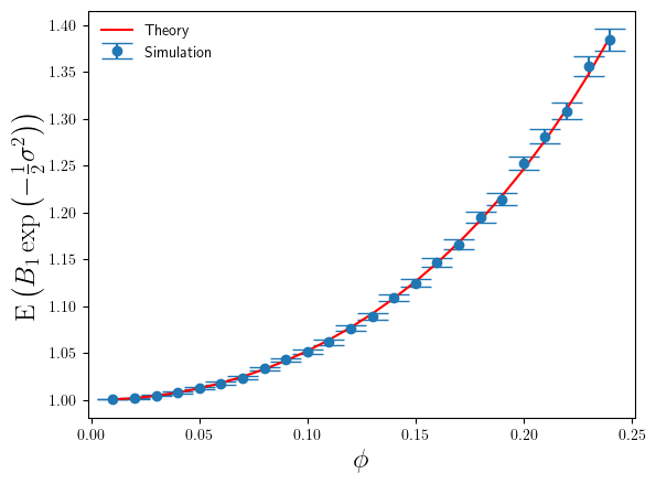
Below in Figure 1 I’ve shown a plot of the expectation of , relative to the true bias correction factor , as a function of . The red line is based on the theoretical calculation in Eq.3, whilst the blue points are simulation estimates,
Figure 1: Plot of theory and simulation estimates of the average relative error made by the parametric bias correction factor, as we increase the variance of the log-normal data.
The agreement between simulation and theory is very good. But even for these small values of we can see the error that makes in estimating the correct bias correction factor is significant – nearly 40% relative error at . For , the value of is 2.24 at . Whilst this is large for the additive log-scale noise, it is not ridiculously large. It shows that the presence of the divergence at is strongly felt even a long way away from that divergence point.
The error bars on the simulation estimates correspond to standard-errors of the mean. In calculating the standard-errors of the mean I’ve used the theoretical calculation of (derived from Eq.5), rather than the simulation sample estimate of it. The reason being that once one goes above about and above , the variance (over different sets of simulation runs) of becomes large itself, and so obtaining a stable accurate simulation estimate of requires such a prohibitively large number of simulations (way greater than 100000) that estimating from a simulation sample becomes impractical. So I used the theoretical result instead. Hence also why the plot below is restricted to .
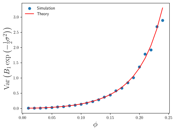
For the range , where the simulation sample size is sufficiently large enough that we can trust our simulation sample based estimates of , we can compare them with the theoretical values. This comparison is plotted in Figure 2 below.
Figure 2: Plot of theory and simulation estimates of the variance of the relative error made by the parametric bias correction factor, as we increase the variance of the log-normal data.
We can see that the simulation estimates of confirm the accuracy of the theoretical result in Eq.5, and consequently confirm the validity of the standard error estimates in Figure 1.
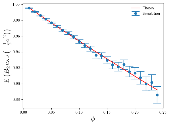
Okay, so that’s confirmed the ‘surprising’ behaviour of the bias-correction estimate , but what about ? How do simulation estimates of and compare to the theoretical results in Eq.4 and Eq.6 ? I’ve plotted these in Figures 3 and 4 below.
Figure 3: Plot of theory and simulation estimates of the average relative error made by the non-parametric bias correction factor, as we increase the variance of the log-normal data.
The accuracy of is much better than that of . By comparison only makes a 10% relative error (under-estimate) on average at , compared to the 40% over-estimate of (on average). We can also see that the magnitude of the relative error increases slowly as increases, again in constrast with the rapid increase in the relative error made by (in Figure 1).
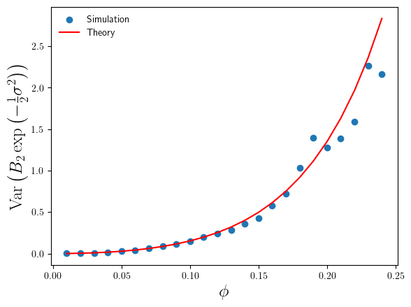
Figure 4: Plot of theory and simulation estimates of the variance of the relative error made by the non-parametric bias correction factor, as we increase the variance of the log-normal data.
Conclusion
So, the theoretical derivations and analysis I did of and turned out to be correct. What did I learn from this? Three things. Firstly, even areas of mathematics that you understand well, have worked with for a long time, and are relatively simple in mathematical terms (e.g. just a univariate distribution) have the capacity to surprise you. Secondly, given this capacity to surprise it is always a good idea to check your mathematical hunches, even with a simple calculation, no matter how confident you are in those hunches. Thirdly, don’t leave it 25 years to check your mathematical hunches. The evaluation of those integrals defining and only took me a couple of minutes. If I had calculated those integrals 25 years ago, I wouldn’t be feeling so stupid now.


![\mathbb{E}\left ( B_{1}\right )\;=\; \left( 2\pi\sigma^{2}\right)^{-\frac{N}{2}}\int_{{\mathbb{R}}^{N}} d{\underline{x}}\exp\left [-\frac{1}{2\sigma^{2}}\left ( \underline{x} - \mu\underline{1}_{N}\right )^{\top}\left ( \underline{x} - \mu\underline{1}_{N}\right )\right ] \exp\left[ \frac{1}{2} \underline{x}^{\top}\underline{\underline{M}}\underline{x}\right ]](https://s0.wp.com/latex.php?latex=%5Cmathbb%7BE%7D%5Cleft+%28+B_%7B1%7D%5Cright+%29%5C%3B%3D%5C%3B+%5Cleft%28+2%5Cpi%5Csigma%5E%7B2%7D%5Cright%29%5E%7B-%5Cfrac%7BN%7D%7B2%7D%7D%5Cint_%7B%7B%5Cmathbb%7BR%7D%7D%5E%7BN%7D%7D+d%7B%5Cunderline%7Bx%7D%7D%5Cexp%5Cleft+%5B-%5Cfrac%7B1%7D%7B2%5Csigma%5E%7B2%7D%7D%5Cleft+%28+%5Cunderline%7Bx%7D+-+%5Cmu%5Cunderline%7B1%7D_%7BN%7D%5Cright+%29%5E%7B%5Ctop%7D%5Cleft+%28+%5Cunderline%7Bx%7D+-+%5Cmu%5Cunderline%7B1%7D_%7BN%7D%5Cright+%29%5Cright+%5D+%5Cexp%5Cleft%5B+%5Cfrac%7B1%7D%7B2%7D+%5Cunderline%7Bx%7D%5E%7B%5Ctop%7D%5Cunderline%7B%5Cunderline%7BM%7D%7D%5Cunderline%7Bx%7D%5Cright+%5D&bg=ffffff&fg=111111&s=0&c=20201002)


![\mathbb{E}\left ( B_{2}\right )\;=\;\frac{1}{N}\sum_{i=1}^{N} \left( 2\pi\sigma^{2}\right)^{-\frac{N}{2}}\int_{{\mathbb{R}}^{N}} d{\underline{x}}\exp\left [-\frac{1}{2\sigma^{2}}\left ( \underline{x} - \mu\underline{1}_{N}\right )^{\top}\left ( \underline{x} - \mu\underline{1}_{N}\right )\right ] \exp \left [ \sum_{j=1}^{N}\left ( \delta_{ij} - \frac{1}{N}\right )x_{j}\right ]](https://s0.wp.com/latex.php?latex=%5Cmathbb%7BE%7D%5Cleft+%28+B_%7B2%7D%5Cright+%29%5C%3B%3D%5C%3B%5Cfrac%7B1%7D%7BN%7D%5Csum_%7Bi%3D1%7D%5E%7BN%7D+%5Cleft%28+2%5Cpi%5Csigma%5E%7B2%7D%5Cright%29%5E%7B-%5Cfrac%7BN%7D%7B2%7D%7D%5Cint_%7B%7B%5Cmathbb%7BR%7D%7D%5E%7BN%7D%7D+d%7B%5Cunderline%7Bx%7D%7D%5Cexp%5Cleft+%5B-%5Cfrac%7B1%7D%7B2%5Csigma%5E%7B2%7D%7D%5Cleft+%28+%5Cunderline%7Bx%7D+-+%5Cmu%5Cunderline%7B1%7D_%7BN%7D%5Cright+%29%5E%7B%5Ctop%7D%5Cleft+%28+%5Cunderline%7Bx%7D+-+%5Cmu%5Cunderline%7B1%7D_%7BN%7D%5Cright+%29%5Cright+%5D%C2%A0+%5Cexp+%5Cleft+%5B+%5Csum_%7Bj%3D1%7D%5E%7BN%7D%5Cleft+%28+%5Cdelta_%7Bij%7D+-+%5Cfrac%7B1%7D%7BN%7D%5Cright+%29x_%7Bj%7D%5Cright+%5D&bg=ffffff&fg=111111&s=0&c=20201002)

![\mathbb{E}\left ( B_{2}\right )\;=\; \exp \left [ \frac{\sigma^{2}}{2}\left ( 1\;-\;\frac{1}{N}\right )\right ]](https://s0.wp.com/latex.php?latex=%5Cmathbb%7BE%7D%5Cleft+%28+B_%7B2%7D%5Cright+%29%5C%3B%3D%5C%3B+%5Cexp+%5Cleft+%5B+%5Cfrac%7B%5Csigma%5E%7B2%7D%7D%7B2%7D%5Cleft+%28+1%5C%3B-%5C%3B%5Cfrac%7B1%7D%7BN%7D%5Cright+%29%5Cright+%5D&bg=ffffff&fg=111111&s=0&c=20201002)


![{\rm Var}\left ( B_{2}\right)\;=\; \left ( 1 - \frac{1}{N}\right )\exp \left [ \sigma^{2}\left ( 1 - \frac{2}{N}\right )\right ]\;+\;\frac{1}{N}\exp \left [ 2\sigma^{2}\left ( 1 - \frac{1}{N}\right )\right ]\;-\; \exp \left [ \sigma^{2}\left ( 1 - \frac{1}{N}\right )\right ]](https://s0.wp.com/latex.php?latex=%7B%5Crm+Var%7D%5Cleft+%28+B_%7B2%7D%5Cright%29%5C%3B%3D%5C%3B+%5Cleft+%28+1+-+%5Cfrac%7B1%7D%7BN%7D%5Cright+%29%5Cexp+%5Cleft+%5B+%5Csigma%5E%7B2%7D%5Cleft+%28+1+-+%5Cfrac%7B2%7D%7BN%7D%5Cright+%29%5Cright+%5D%5C%3B%2B%5C%3B%5Cfrac%7B1%7D%7BN%7D%5Cexp+%5Cleft+%5B+2%5Csigma%5E%7B2%7D%5Cleft+%28+1+-+%5Cfrac%7B1%7D%7BN%7D%5Cright+%29%5Cright+%5D%5C%3B-%5C%3B+%5Cexp+%5Cleft+%5B+%5Csigma%5E%7B2%7D%5Cleft+%28+1+-+%5Cfrac%7B1%7D%7BN%7D%5Cright+%29%5Cright+%5D&bg=ffffff&fg=111111&s=0&c=20201002)