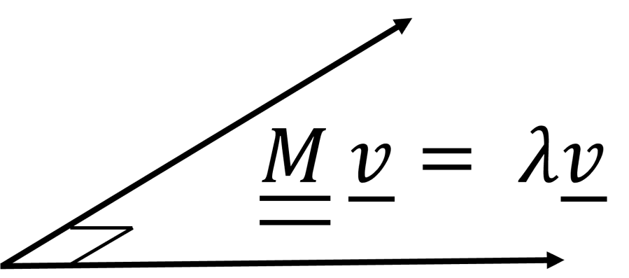
Data Science Notes: 6. Finding eigenvectors by hand

In another post I had to find the eigenvalues and eigenvectors of the following matrix,

\underline{\underline{M}}\;=\; a\underline{\underline{I}}_{N} + b\underline{1}_{N}\underline{1}_{N}^{\top}    Eq.1

where \underline{1}_{N} is an N-dimensional vector with elements all 1, whilst \underline{\underline{I}}_{N} is the N\times N identity matrix.

In that original post I said that diagonalizing this matrix (finding its eigenvalues and eigenvectors) was easy. A colleague asked me why I thought it was easy. My answer, “well because it is the only matrix form whose eigen-decomposition I explicitly remember”. And there’s a reason why I remember how to decompose by hand these types of matrices,

  1. It is easy to do.
  2. These types of matrices are very common.

Okay, I know that reason 1 is a circular argument, but it’s true. These types of matrices are easy to diagonalize and you’ll agree when you learn the trick to calculate their eigenvalues and eigenvectors. And like all the posts in my Data Science Notes series, I’m basing this post on experience. It is nearly 29 years since I first learnt this trick, and I have used it many time since. The reason I find it so useful is because of reason 2 above.

Reason 2 is equally important. As a Data Scientist you will encounter this form of matrix often, and so there is an advantage to knowing how to calculate the eigenvectors and eigenvalues of a matrix such as \underline{\underline{M}} in Eq.1, and you learn a lot about eigenvectors and eigenvalues in doing so; you learn what they are, what they represent, how to manipulate them, and how to use them to do useful things. We can view the matrix \underline{\underline{M}} in Eq.1 as a low-rank perturbation of the identity matrix, and manipulating matrices by adding a low-rank perturbation is a common trick in the mathematical and statistical sciences, most recently used in LoRA (low-rank adaptation) algorithms for fine-tuning Large Language Models (LLMs). So getting comfortable with the mathematics of eigen-decompositions of low-rank perturbations will pay off.

Let’s begin. To start we’ll need to do a quick recap of what an eigenvector is and what an eigenvalue is.

Recap of what eigenvectors and eigenvalues are

An eigenvector \underline{v} of a square matrix \underline{\underline{M}} is a vector that satisfies the following equation,

\underline{\underline{M}}\, \underline{v}\;=\; \lambda \underline{v}     Eq.2

The scalar quantity \lambda is the eigenvalue corresponding to the eigenvector \underline{v}. Given a vector \underline{v} that satisfies Eq.2, then the vector a\underline{v} also satisfies Eq.2 for any choice of the scalar a. This means we have the freedom to set the norm of the vector \underline{v} since we can effectively absorb the effect of any choice of norm into the effective value of a. So without loss of generality we can set \underline{v}^{\top}\underline{v}\;=\;1.

An N \times N matrix will have N different eigenvectors, some of which may have the same eigenvalue. So overall we have a set \{\underline{v}_{k}\}_{k=1}^{N} of eigenvectors with corresponding eigenvalues \{\lambda_{k}\}_{k=1}^{N}. Eigenvectors corresponding to eigenvalues that have different values are orthogonal to each other. Eigenvectors corresponding to the same eigenvalue need not be orthogonal to each other, but we can always construct an orthonormal set that spans the same subspace, so without loss of generality we can take the set of eigenvectors \{\underline{v}_{k}\}_{k=1}^{N} to form an orthonormal set.

The eigen-decomposition of a matrix

We can see from Eq.2 that the effect of the matrix \underline{\underline{M}} on an eigenvector \underline{v} is simply to multiply it by a scale factor \lambda. Consequently, the eigenvectors of a matrix are very special. In fact they allow us to characterize or represent the matrix \underline{\underline{M}} in the following way,

\underline{\underline{M}}\;=\; \sum_{k=1}^{N}\lambda_{k} \underline{v}_{k}\,\underline{v}_{k}^{\top}   Eq.3

And once we have all the eigenvectors \{\underline{v}\}_{k=1}^{N} and corresponding eigenvalues \{\lambda_{k}\}_{k=1}^{N} of a matrix \underline{\underline{M}} we can do useful things such as calculate its inverse or calculate its determinant, which occur in multiple places in multi-variate statistics, machine learning, and GenAI. I also needed them for the calculations in my original blog-post . The inverse and determinant of \underline{\underline{M}} are given by the usual formulae,

\underline{\underline{M}}^{-1}\;=\;\sum_{k=1}^{N}\lambda_{k}^{-1}\underline{v}_{k}\,\underline{v}_{k}^{\top}   Eq.4

\det \underline{\underline{M}}\;=\;\prod_{k=1}^{N}\lambda_{k}    Eq.5

Identifying our eigenvectors

Now, our goal is the work out the eigenvalues and eigenvectors of the matrix,

\underline{\underline{M}} \;=\; a_{0}\underline{\underline{I}}_{N} + \sum_{k=1}^{K} a_{k}\underline{u}_{k}\underline{u}_{k}^{\top}     Eq.6

In Eq.6 I have generalized from the matrix form in Eq.1 a little here, so we have 1 \leq K \ll N vectors \underline{u}_{k}, k=1,\ldots,K, which form an orthonormal set, i.e. they are all of unit length and orthogonal to each other.

Let’s write the right-hand-side of Eq. 6 as a sum of two matrices, i.e. we write, \underline{\underline{M}} in Eq.6 as,

\underline{\underline{M}} = a_{0}\underline{\underline{I}}_{N} \;+\; \underline{\underline{A}}    Eq. 7,

with the matrix \underline{\underline{A}} defined as,

\underline{\underline{A}}\;=\; \sum_{k=1}^{K} a_{k}\underline{u}_{k}\underline{u}_{k}^{\top}    Eq.8

This leads us to our first trick. If we have a vector \underline{v} which is an eigenvector of \underline{\underline{A}} with eigenvalue \lambda, then we can easily work out the effect of \underline{\underline{M}} on \underline{v} because the identity matrix \underline{\underline{I}} leaves \underline{v} unchanged. So overall we have,

\underline{\underline{M}}\, \underline{v}\;=\; \left ( a_{0}\underline{\underline{I}} + \underline{\underline{A}} \right )\, \underline{v}\;=\; a_{0}\underline{\underline{I}}\, \underline{v} \;+\; \underline{\underline{A}}\, \underline{v}\;=\; \left ( a_{0} + \lambda \right ) \underline{v}     Eq. 9

Eq.9 tells us that eigenvectors of \underline{\underline{A}} are eigenvectors of \underline{\underline{M}}. We only need to find eigenvectors and eigenvalues of \underline{\underline{A}}.

Now we introduce our second trick. We look at the definition of \underline{\underline{A}} in Eq. 8 and compare it to the eigen-decomposition in Eq.3. They are of the same form. Matrix \underline{\underline{A}} is already in the form an eigen-decomposition. The vectors \underline{u}_{k} are the eigenvectors \underline{\underline{A}}. And the corresponding eigenvalues are a_{k}.

Ok, but we only have K vectors \underline{u}_{k} and we need N eigenvectors. Easy, consider any vector, \underline{v} that is orthogonal to all the vectors \{\underline{u}_{k}\}_{k=1}^{K}. The effect of \underline{\underline{A}} on that vector \underline{v} is as follows,

\underline{\underline{A}}\, \underline{v} \;=\; \underline{0}    Eq.10

So any vector orthogonal to all the vectors \{\underline{u}_{k}\}_{k=1}^{K} will be an eigenvector of \underline{\underline{A}} with an eigenvalue of zero.

Now we can combine our first and second tricks together the finally work out the eigenvectors and eigenvalues of \underline{\underline{M}}. These are,

Eigenvalue = a_{0} + a_{1} , Eigenvector = \underline{u}_{1}
Eigenvalue = a_{0} + a_{2}, Eigenvector = \underline{u}_{2}
……
Eigenvalue = a_{0} + a_{K}, Eigenvector = \underline{u}_{K}
Eigenvalue = a_{0} , Eigenvectors = Any orthonormal set that spans the subspace orthogonal to the vectors \{\underline{u}_{k}\}_{k=1}^{K}.

Putting it all together

Let’s put this into action. Let’s go back to our original matrix in Eq.1 at the start of this post. That matrix was of the form,

\underline{\underline{M}}\;=\; a\underline{\underline{I}}_{N} + b\underline{1}_{N}\underline{1}_{N}^{\top}    Eq.11

So comparing Eq.11 to Eq.6 we have a_{0} = a, K=1, \underline{u}_{1} = \frac{1}{\sqrt{N}}\underline{1}_{N}, and a_{1} = Nb. So our eigenvectors and corresponding eigenvalues are,

Eigenvalue 1 = a + Nb , Eigenvector 1 = \frac{1}{\sqrt{N}}\underline{1}_{N}
Eigenvalues 2 to N = a , Eigenvectors 2 to N = an orthonormal set orthogonal to \underline{1}_{N} .

We can now easily calculate the determinant of our matrix in Eq.1 and we get,

\det \underline{\underline{M}}\;=\;(a+Nb)a^{N-1}     Eq.12

We can also easily calculate the inverse of the matrix in Eq.1. In this case we get,

\underline{\underline{M}}^{-1}\;=\;\sum_{k=2}^{N}\frac{1}{a}\underline{v}_{k}\underline{v}_{k}^{\top}\;+\; \frac{1}{(a+Nb)N}\underline{1}_{N}\underline{1}_{N}^{\top}     Eq.13

In Eq.13 the vectors \underline{v}_{k}\; ,\;k=2,\ldots, N form an orthonormal set orthogonal to \underline{1}_{N}.

Now, we can use one final little trick to simplify the right-hand-side of Eq.13. If we recall that the effect of the identity matrix \underline{\underline{I}}_{N} on any vector v_{k} from an orthonormal set \{\underline{v}_{k}\}_{k}^{N} is to leave those vectors unchanged, then this means we can write the identity matrix \underline{\underline{I}}_{N} in terms of an eigen-decomposition, and that decomposition is as follows,

\underline{\underline{I}}_{N}\;=\; \sum_{k=1}^{N}\underline{v}_{k}\underline{v}_{k}^{\top}     Eq.14

Now Eq.14 is almost what we have in the first term on the right-hand-side of Eq.13. Our sum in Eq.13 runs from k=2 to k=N, whilst the sum in Eq.14 runs from k=1 to k=N. If only we had another vector \underline{v}_{1} that was orthogonal to \underline{v}_{2}, \underline{v}_{3} etc.? But we do! We have \frac{1}{\sqrt{N}}\underline{1}_{N}. In fact, that is how we defined \underline{v}_{2}, \underline{v}_{3} etc. – they are all orthogonal to \frac{1}{\sqrt{N}}\underline{1}_{N}. This means if we set \underline{v}_{1} = \frac{1}{\sqrt{N}}\underline{1}_{N}, we can re-write the sum in the right-hand-side of Eq.13 as,

\sum_{k=2}^{N}\frac{1}{a}\underline{v}_{k}\underline{v}_{k}^{\top}\;=\; \frac{1}{a}\sum_{k=2}^{N}\underline{v}_{k}\underline{v}_{k}^{\top}\;+\; \frac{1}{aN} \underline{1}_{N}\underline{1}_{N}^{\top}\;-\; \frac{1}{aN} \underline{1}_{N}\underline{1}_{N}^{\top}
=\; \frac{1}{a}\sum_{k=1}^{N} \underline{v}_{k}\underline{v}_{k}^{\top}\;-\;\frac{1}{aN} \underline{1}_{N}\underline{1}_{N}^{\top}    Eq.15

where the vectors \underline{v}_{1}, \underline{v}_{2},\underline{v}_{3} etc. form an orthonormal set in \mathbb{R}^{N}. This means (by comparing to Eq.14) we can also write the last expression in Eq.15 as,

\frac{1}{a}\underline{\underline{I}}_{N}\;-\;\frac{1}{aN} \underline{1}_{N}\underline{1}_{N}^{\top}     Eq.16

Combining this with the final term on the right-hand-side of Eq.13 we get our final simplified expression for \underline{\underline{M}}^{-1}, which is,

\underline{\underline{M}}^{-1}\;=\; \frac{1}{a}\underline{\underline{I}}_{N}\;-\; \frac{b}{a(a+Nb)}\underline{1}_{N}\underline{1}_{N}^{\top}     Eq.17

That’s it. If you want a challenge to test your understanding, then using the ideas and tricks we introduced above see if you can construct a closed form expression for the inverse of the matrix in Eq.6, not just the special case of the matrix in Eq.1.

Other low-rank perturbation tricks

In my original post I wanted to find the eigenvectors and eigenvalues of the matrix in Eq.1. I’ve also illustrated that once we have closed-form expressions for the eigenvectors and eigenvalues we can calculate the determinant and inverse of \underline{\underline{M}} in Eq.1 very easily. But it is also worth pointing out that there are a couple of other tricks for evaluating the determinant and inverse of matrices of the form in Eq.1 and Eq.6, namely,

  1. Sylvester’s determinant theorem. The Wikipedia link here is for the Weinstein–Aronszajn identity as it turns out that the deteminant theorem has been mis-attributed to Sylvester – I was taught it as Sylvester’s theorem in university. This allows us to calculate the determinant of a low-rank pertubation in terms of a determinant of a smaller matrix.
  2. The Woodbury formula. This allows us to express the inverse of a low-rank perturbation in terms of matrix multiplications involving the inverse of the unperturbed matrix. In fact the result in Eq.17 can also be obtained by using the Shermann-Morrison formula, which is a special case of the Woodbury formula.

Sylvester’s theorem and the Woodbury formula only give us information about the determinant and inverse of the low-rank perturbation, so if we explicitly want information about the eigenvectors and eigenvalues we will probably have to use the tricks I have outlined in this post. However, the advantage of the Sylvester and Woodbury formulae is that they can be used when we have a base-case (the unperturbed matrix) that isn’t necessarily the identity matrix, i.e. they are more widely applicable than the tricks I’ve outlined in this post. What the Sylvester and Woodbury formulae also illustrate is that we shouldn’t be frightened of working with low-rank perturbations of base-case matrices. Once you learn a few tricks working with them becomes very easy.

What have we learnt?

  1. How to calculate analytically (by hand) the eigenvectors and eigenvalues of matrices of the form in Eq.6.
  2. But more importantly, we’ve learnt along the way that eigenvectors and eigenvalues are not that scary. They are easy to manipulate and work with once you get comfortable with a few concepts that you have probably already learnt at college or at university. Matrices of the form in Eq.6 are the simplest, realistic matrices which bring those concepts to life. These matrices are a great learning ground.
  3. Even better, matrices of the type in Eq.6 occur a lot in Data Science, Machine Learning, and AI. In fact, it is probably one of Data Science’s secrets; 95% or more of Data Scientists, myself included, stick to using matrices of this form or a low-rank perturbation of some other known base-case matrix when modelling a real problem. And why not!? When modelling a real problem we start with the base-case we understand and change it as little as possible, both for model complexity reasons (number of extra parameters etc.) and for reasons of computational complexity (can we easily compute and understand the properties of the new matrix). So if you get comfortable working with eigenvectors and eigenvalues of low-rank perturbations of simple base-case matrices, you’ve cracked it for 95% of Data Science use-cases.


© 2026 David Hoyle. All Rights Reserved

Log Normal Bias and the infinite capacity of mathematics to surpise

Summary

  • Always confirm your mathematical intuition with an explicit calculation, no matter how simple the calculation.
  • Always confirm your mathematical intuition with an explicit calculation, no matter how well you know the particular area of mathematics.
  • Don’t leave it 25 years to check your mathematical intuition with a calculation, no matter how confident you are in that intuition.

Introduction

One of the things about mathematics is that it’s not afraid to slap you in the face and stand there laughing at you. Metaphorically speaking, I mean. Mathematics has an infinite capacity to surprise even in areas where you think you can’t be surprised. And you end up looking or feeling like an idiot, with mathematics laughing at you.

This is a salutary lesson about how I thought I understood an area of statistics, but didn’t. The area in question is the log-normal distribution. This is a distribution I first encountered 25 years ago and have worked with almost continuously since.

The problem which slapped me in the face

The particular aspect of the log-normal distribution in question, was what happens when you go from models or estimates on the log-scale, to models or estimates on the ‘normal’ or exponentiated scale. For a log-normal random variable Y with \sigma^{2} being the variance of \log Y, we have the well-known result,

\mathbb{E}\left ( Y \right ) \;=\; \exp\left( \mathbb{E}\left (\log Y \right ) \right ) \times \exp\left ( \frac{1}{2}\sigma^{2}\right )

This is an example of Jensen’s inequality at work. If you apply a non-linear function f to a random variable Y, then the average of the function is not equal to the function of the average. That is, \mathbb{E}\left ( f(Y)\right )\;\neq\; f\left ( \mathbb{E}\left ( Y\right )\right ).

In the case of the log-normal distribution, the first equation above tells us that we can relate the \mathbb{E}\left ( \log Y\right ) to \mathbb{E}\left (Y)\right) via a simple bias-correction factor \exp ( \frac{1}{2}\sigma^{2} ). So, if we had a sample of N observations of \log Y we could estimate the expectation of Y from an estimate of the expectation of \log Y by multiplying by a bias correction factor of \exp\left ( \frac{1}{2} \sigma^{2}\right ). We can estimate \sigma^{2} from the residuals of our estimate of the expectation of \log Y. In this case, I’m going to assume our model is just an estimation of the mean, \mathbb{E}\left ( \log Y \right ), which I’ll denote by \mu, and I’m not going to try to decompose \mu any further. If our estimate of \mu is just the sample mean of \log Y, then our estimate of \sigma^{2} would simply be the sample variance, s^{2}. If we denote our observations by y_{i}\;,\; i=1,\ldots,N then s^{2} is given by the formula,

s^{2}\;=\; \frac{1}{N-1}\sum_{i} \log^{2} y_{i} \;-\;  \frac{1}{N(N-1)}\left( \sum_{i}\log y_{i}\right )^{2}

Note the usual Bessel correction that I’ve applied in the calculation of s^{2}.

We can see from this discussion that the bias correction in going from the log-scale to the ‘normal’ scale is multiplicative in this case. The bias correction factor B_{1} is given by,

B_{1} \;=\;\exp\left ( \frac{1}{2}  s^{2}\right )

If we had suspected that any bias correction needs to be multiplicative, which seems reasonable given we are going from a log-scale to a normal-scale, then we could easily have estimated a bias correction factor as simply the ratio of the mean of the observations on the normal scale to the exponential of the mean of the observations on the log scale. That is, we can construct a second estimate, B_{2}, of the bias correction factor needed, with B_{2} given by,

B_{2} \; =\; \frac{\frac{1}{N}\sum_{i}y_{i}}{\exp\left ( \frac{1}{N}\sum_{i}\log y_{i}\right )}

I tend to refer to the B_{2} method as a non-parametric method because it is how you would estimate \mathbb{E}\left ( Y \right ) from an estimate of \mathbb{E}\left ( \log Y \right ) and you only knew the bias correction needed was multiplicative. You wouldn’t explicitly need to make any assumptions about the distribution of the data. In contrast, B_{1} is specific to the data coming from a log-normal distribution, so I call it a parametric estimate. For these reasons, I tend to prefer using the B_{2} way of estimating any necessary bias correction factor, as obviously any real data won’t be perfectly log-normal and so the B_{2} estimator will be more robust whilst also being very simple to calculate.

A colleague asks an awkward question

So far everything I’ve described is well known and pretty standard. However, a few months ago a colleague asked me if there would be any differences between the estimates B_{1} and B_{2}? “Of course”, I said, if the data is not log-normal. “No”, my colleague said. They meant, even if the data was log-normal would there be any differences between the estimates B_{1} and B_{2}. Understanding the size of any differences when the parametric assumptions are met would help understand how big the differences could be when the parametric assumptions are violated. “Yeah, there will obviously still be differences between B_{1} and B_{2} even if we do have log-normal data, because of sampling variation affecting the two formulae differently. But, I would expect those differences to be small even for moderate sample sizes”, I confidently replied.

I’ve been using those formulae for B_{1} and B_{2} for over 25 years and never considered the question my colleague asked. I’d never confirmed my intuition. So 25 years later, I thought I’d do a quick calculation to confirm my intuition. My intuition was very very wrong! I thought it would be interesting to explain the calculations I did and what, to me, was the surprising behaviour of B_{1}. Note, with hindsight the behaviour I uncovered shouldn’t have been surprising. It was obvious once I’d begun to think about it. It was just that I’d left thinking about it till 25 years too late.

The mathematical detail

The question my colleague was asking was this. If we have N i.i.d. observations drawn from a log-normal distribution, i.e.,

x_{i}\;=\;\log y_{i} \sim {\cal{N}}\left (\mu, \sigma^{2}\right )\;\;\;   , i = 1,\ldots,N\;\;\;,

what are the expectation values of the bias correction factors B_{1} and B_{2} at any finite value of N. Do \mathbb{E}\left ( B_{1} \right ) and \mathbb{E}\left ( B_{2}\right ) converge to \exp(\frac{1}{2}\sigma^{2}) as N\rightarrow\infty, and if so how fast?

Since the \log y_{i} are Gaussian random variables we can express these expectation values in terms of simple integrals and we get,

\mathbb{E}\left ( B_{1}\right )\;=\; \left( 2\pi\sigma^{2}\right)^{-\frac{N}{2}}\int_{{\mathbb{R}}^{N}} d{\underline{x}}\exp\left [-\frac{1}{2\sigma^{2}}\left ( \underline{x} - \mu\underline{1}_{N}\right )^{\top}\left ( \underline{x} - \mu\underline{1}_{N}\right )\right ] \exp\left[ \frac{1}{2} \underline{x}^{\top}\underline{\underline{M}}\underline{x}\right ]   Eq.1

where the matrix \underline{\underline{M}} is given by,

\underline{\underline{M}}\;=\;\frac{1}{N-1}\underline{\underline{I}}_{N}\;-\;\frac{1}{N(N-1)}\underline{1}_{N}\underline{1}_{N}^{\top}.

Here {\underline{1}}_{N} is an N-dimensional vector consisting of all ones, and \underline{\underline{I}}_{N} is the N\times N identity matrix.

We can similarly express the expectation of B_{2} and we get,

\mathbb{E}\left ( B_{2}\right )\;=\;\frac{1}{N}\sum_{i=1}^{N} \left( 2\pi\sigma^{2}\right)^{-\frac{N}{2}}\int_{{\mathbb{R}}^{N}} d{\underline{x}}\exp\left [-\frac{1}{2\sigma^{2}}\left ( \underline{x} - \mu\underline{1}_{N}\right )^{\top}\left ( \underline{x} - \mu\underline{1}_{N}\right )\right ]  \exp \left [ \sum_{j=1}^{N}\left ( \delta_{ij} - \frac{1}{N}\right )x_{j}\right ]   Eq.2

The matrices in the exponents of the integrands of Eq.1 and Eq.2 are easily diagonalized analytically and so the integrals are relatively easy to evaluate analytically. From this we find,

\mathbb{E}\left ( B_{1}\right )\;=\; \left ( 1\;\;-\;\frac{\sigma^{2}}{N-1}\right )^{-\frac{(N-1)}{2}}  Eq.3

\mathbb{E}\left ( B_{2}\right )\;=\; \exp \left [ \frac{\sigma^{2}}{2}\left ( 1\;-\;\frac{1}{N}\right )\right ]   Eq.4

We can see that as N\rightarrow\infty both expressions for the bias correction tend to the correct value of \exp(\sigma^2/2). However, what is noticeable is at finite N the value of \mathbb{E}\left( B_{1}\right)) has a divergence. Namely, as \sigma^{2} \rightarrow N-1, we have \mathbb{E}\left( B_{1}\right ) \rightarrow \infty and for \sigma^{2} \ge N-1, we have that \mathbb{E}\left( B_{1}\right ) doesn’t exist. This means that for a finite sample size there are situations where the parametric form of the bias correction will be very very wrong.

At first sight I was shocked and surprised. The divergence shouldn’t have been there. But it was. My intuition was wrong. I was expecting there to be differences between \mathbb{E}\left ( B_{1}\right) and \mathbb{E}\left ( B_{2}\right ), but very small ones. I’d largely always thought of any large differences that arise in practice between the two methods to be due to the distributional assumption made –  because a real noise process won’t follow a log-normal distribution we’ll always get some differences. But the derivations above are analytic. They show that there can be a large difference between the two bias-correction estimation methods even when all assumptions about the data have been met.

With hindsight, the reason for the large difference between the two expectations is obvious. The second, \mathbb{E}\left ( B_{2}\right ), involves the expectation of the exponential of a sum of Gaussian random variables, whilst the first involves the expectation of the exponential of a sum of the squares of those same Gaussian random variables. The expectation in Eq.1 is a Gaussian integral and if \sigma^{2} is large enough the coefficient of the quadratic term in the exponent becomes positive, leading to the expectation value becoming undefined.

Even though in hindsight the result I’d just derived was obvious, I still decided to simulate the process to check it. As part of the simulation I also wanted to check the behaviour of the variances of B_{1} and B_{2}, so I needed to derive analytical results for {\rm Var}\left ( B_{1}\right ) and {\rm Var}\left ( B_{2}\right ). These calculations are similar to the evaluation of \mathbb{E}\left ( B_{1}\right ) and \mathbb{E}\left ( B_{2}\right ), so I’ll just state the results below,

{\rm Var}\left ( B_{1}\right)\;=\; \left ( 1 - \frac{2\sigma^{2}}{N-1}\right )^{-\frac{(N-1)}{2}}\;-\;\left ( 1 - \frac{\sigma^{2}}{N-1} \right )^{-(N-1)}  Eq.5

{\rm Var}\left ( B_{2}\right)\;=\; \left ( 1 - \frac{1}{N}\right )\exp \left [ \sigma^{2}\left ( 1 - \frac{2}{N}\right )\right ]\;+\;\frac{1}{N}\exp \left [ 2\sigma^{2}\left ( 1 - \frac{1}{N}\right )\right ]\;-\; \exp \left [ \sigma^{2}\left ( 1 - \frac{1}{N}\right )\right ]  Eq.6

Note that the variance of B_{1} also diverges, but when \frac{\sigma^{2}}{N-1} = \frac{1}{2}, so much before \mathbb{E}\left ( B_{1}\right ) diverges.

To test Eq.3 – Eq.6 I ran some simulations. First, I introduced a scaled variance \phi = \sigma^{2}/(N-1). The divergence in \mathbb{E}\left ( B_{1}\right ) occurs at \phi = 1, so \phi gives us a way of measuring how problematic the value of \sigma^{2} will be for the given value of N. The divergence in {\rm Var}\left ( B_{1} \right ) occurs at \phi = 0.5. I chose to set N=20 in my simulations, so quite a small sample but there are good reasons that I’ll explain later. For each value of \phi I generated N_{sim} = 100000 sample datasets, each of N log-normal datapoints, and calculated B_{1} and B_{2}. From the simulation sample of B_{1} and B_{2} values I then calculated sample estimates of \mathbb{E}\left ( B_{1}\right ), \mathbb{E}\left ( B_{2}\right ), {\rm Var}\left ( B_{1}\right ), and {\rm Var}\left ( B_{2}\right ). The simulation code is in the Jupyter notebook LogNormalBiasCorrection.ipynb in the GitHub repository here.

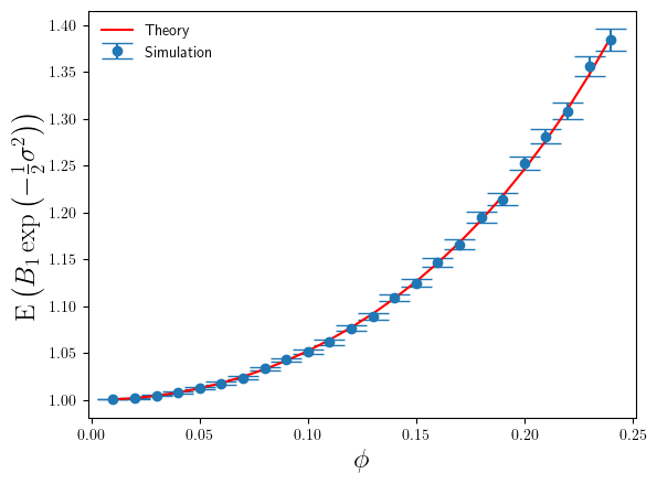
Below in Figure 1 I’ve shown a plot of the expectation of B_{1}, relative to the true bias correction factor \exp\left( \frac{1}{2}\sigma^{2}\right ), as a function of \phi. The red line is based on the theoretical calculation in Eq.3, whilst the blue points are simulation estimates,

A plot showing how the average relative error made by the parametric bias correction factor increases as the variance of the log-normal data increases. The plot shows both simulation and theory estimates of the relative error. The theory is in close agreement with the simulation results.
Figure 1: Plot of theory and simulation estimates of the average relative error made by the parametric bias correction factor, as we increase the variance of the log-normal data.

The agreement between simulation and theory is very good. But even for these small values of \phi we can see the error that B_{1} makes in estimating the correct bias correction factor is significant – nearly 40% relative error at \phi = 0.25. For N=20, the value of \sigma is 2.24 at \phi=0.25. Whilst this is large for the additive log-scale noise, it is not ridiculously large. It shows that the presence of the divergence at \phi = 1 is strongly felt even a long way away from that divergence point.

The error bars on the simulation estimates correspond to \pm 2 standard-errors of the mean. In calculating the standard-errors of the mean I’ve used the theoretical calculation of {\rm Var}\left ( B_{1}\exp\left ( -\frac{1}{2}\sigma^{2}\right )\right ) (derived from Eq.5), rather than the simulation sample estimate of it. The reason being that once one goes above about N=20 and above \phi = 0.25, the variance (over different sets of simulation runs) of {\rm Var}\left ( B_{1}\exp\left ( -\frac{1}{2}\sigma^{2}\right )\right ) becomes large itself, and so obtaining a stable accurate simulation estimate of {\rm Var}\left ( B_{1}\exp\left ( -\frac{1}{2}\sigma^{2}\right )\right ) requires such a prohibitively large number of simulations (way greater than 100000) that estimating {\rm Var}\left ( B_{1}\exp\left ( -\frac{1}{2}\sigma^{2}\right )\right ) from a simulation sample becomes impractical. So I used the theoretical result instead. Hence also why the plot below is restricted to \phi \le 0.25.

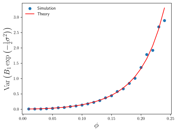
For the range \phi\le 0.25, where the simulation sample size is sufficiently large enough that we can trust our simulation sample based estimates of {\rm Var}\left ( B_{1}\exp\left ( -\frac{1}{2}\sigma^{2}\right )\right ), we can compare them with the theoretical values. This comparison is plotted in Figure 2 below.

A plot showing how variance of the relative error made by the parametric bias correction factor increases as the variance of the log-normal data increases. The plot shows both simulation and theory estimates of the relative error. The theory is in close agreement with the simulation results.
Figure 2: Plot of theory and simulation estimates of the variance of the relative error made by the parametric bias correction factor, as we increase the variance of the log-normal data.

We can see that the simulation estimates of {\rm Var}\left ( B_{1}\exp\left ( -\frac{1}{2}\sigma^{2}\right )\right ) confirm the accuracy of the theoretical result in Eq.5, and consequently confirm the validity of the standard error estimates in Figure 1.

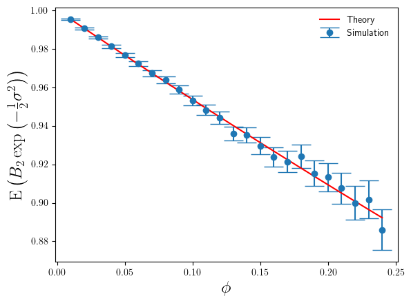
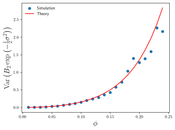
Okay, so that’s confirmed the ‘surprising’ behaviour of the bias-correction estimate B_{1}, but what about B_{2}? How do simulation estimates of  \mathbb{E}\left ( B_{2}\right ) and {\rm Var}\left ( B_{2}\exp\left ( -\frac{1}{2}\sigma^{2}\right )\right ) compare to the theoretical results in Eq.4 and Eq.6 ? I’ve plotted these in Figures 3 and 4 below.

A plot showing how the average relative error made by the non-parametric bias correction factor changes as the variance of the log-normal data increases. The plot shows both simulation and theory estimates of the relative error. The theory is in close agreement with the simulation results.
Figure 3: Plot of theory and simulation estimates of the average relative error made by the non-parametric bias correction factor, as we increase the variance of the log-normal data.

The accuracy of B_{2} is much better than that of B_{1}. By comparison B_{2} only makes a 10% relative error (under-estimate) on average at \phi=0.25, compared to the 40% over-estimate of B_{1} (on average). We can also see that the magnitude of the relative error increases slowly as \phi increases, again in constrast with the rapid increase in the relative error made by B_{1} (in Figure 1).

A plot showing how variance of the relative error made by the non-parametric bias correction factor increases as the variance of the log-normal data increases. The plot shows both simulation and theory estimates of the relative error. The theory is in close agreement with the simulation results.
Figure 4: Plot of theory and simulation estimates of the variance of the relative error made by the non-parametric bias correction factor, as we increase the variance of the log-normal data.

Conclusion

So, the theoretical derivations and analysis I did of B_{1} and B_{2} turned out to be correct. What did I learn from this? Three things. Firstly, even areas of mathematics that you understand well, have worked with for a long time, and are relatively simple in mathematical terms (e.g. just a univariate distribution) have the capacity to surprise you. Secondly, given this capacity to surprise it is always a good idea to check your mathematical hunches, even with a simple calculation, no matter how confident you are in those hunches. Thirdly, don’t leave it 25 years to check your mathematical hunches. The evaluation of those integrals defining \mathbb{E}\left ( B_{1}\right ) and \mathbb{E}\left ( B_{2}\right ) only took me a couple of minutes. If I had calculated those integrals 25 years ago, I wouldn’t be feeling so stupid now.

© 2026 David Hoyle. All Rights Reserved

The shape of mathematics to come

Summary

  • Using AI for mathematics research is a much less hyped field than GenAI in general.
  • The pre-print, “The Shape of Math To Come”, from Alex Kontorovich gives an excellent recent, readable, and accessible discussion of the potential for using AI to scale-up and automate formal mathematics research.

Introduction

Like the rest of the universe I’ve been drawn into experimenting with GenAI for general productivity tasks. However, one of my other interests is how GenAI gets used in scientific discovery. Even more interesting is how GenAI can be used in mathematical discovery. If you want to know where the combination of mathematics and AI is going or could go, then I would strongly recommend reading this arXiv pre-print from Alex Kontorovich, titled “The Shape of Math To Come”. The pre-print was uploaded to the archive in October of this year. With some free evenings last week, I finally got round to finish reading and digesting it.

GenAI for rigorous mathematics? Really?

It’s important to point out that I’m not talking about the mathematics behind GenAI, but about how GenAI is used or could be used as a tool to support the formal development of rigorous mathematical proofs, derivations and statements. Because of that rigour, there is actually less hype (compared to mainstream applications of GenAI) around the use of AI in this way. In the pre-print Kontorovich outlines a credible and believable road ahead for using GenAI in formal mathematics. For me the roadmap is credible because of i)Kontorovich’s credentials as Distinguished Professor of mathematics at Rutger’s University, ii) the significant progress that has been made in this area over the last couple of years, particularly the AlphaProof system from DeepMind, iii) and the existence of powerful automated theorem provers such as Lean.

The pre-print is very readable and even if you don’t have a formal mathematical background but have, say an undergraduate science or engineering degree, you will be able to follow the majority of the discussion – there is only one place where specialized knowledge of analysis is used and even then it is not essential for following Kontorovich’s argument.

The main potential sticking point that Kontorovich highlights in using AI to do maths is the tension between the stochastic nature of Large Language Models (LLMs) and the deterministic nature of mathematical proof. Kontorovich’s argument is that the use of automated theorem checkers such as Lean, in combination with a large and increasing library (MathLib) that formally encodes our current rigorous mathematical knowledge base, will provide a checking mechanism to mitigate the stochastic nature of LLM outputs. In this scenario, human mathematicians are elevated to the role of orchestrating and guiding the LLMs in their attempts to construct new proofs and derivations (using Lean and aided by the knowledge base encoded in MathLib). Whether human mathematicians choose to adopt this approach will depend on how fruitful and easy to use the new GenAI-based mathematics tools are. By analogy with the take-up of the LaTeX typesetting language in the early 1990s, Kontorovich says that this will be when “the ratio of time required to discover and formalize a mathematical result (from initial idea through verified formal proof) to the time required to discover and write up the same result in natural language mathematics” falls below one. When this happens there will also be accelerated ‘network’ effects – increased number of verified proofs encoded into MathLib will increase the ability of computer + GenAI assisted workflows to construct further verified proofs.

Less formal mathematics research

What interests me as a Data Scientist is, if such approaches are successful in advancing how mathematicians do formal mathematics, how much of those approaches can be adopted or modified to advance how non-mathematicians do non-formal mathematics. I’m not talking about the “closed-loop” GenAI-based “robot scientist” approaches that are being discussed in drug-discovery and materials development fields. I’m talking about the iterative, exploratory process of developing a new model training algorithm for a new type of data, or new application domain, or new type of problem. Data Science is typically about approximation. Yes, there is formal derivation in places, and rigorous proofs in others, but there is also a lot of heuristics. Those heuristics can be expressed mathematically, but they are still heuristics. This is not a criticism of using such heuristics – sometimes they are used out of ignorance that better approaches exist, but often they are used out of necessity arising from constraints imposed by the scale of the problem or runtime and storage constraints. What I’m driving at is that the Data Science development process is a messy workflow, with some steps being highly mathematical and imposing a high degree of rigour, some less so. Having access to proven tools that accelerate the exploration of the mathematical steps of that workflow can obviously accelerate the overall Data Science development process. At the moment, switching between mathematical and non-mathematical steps introduces context-switching and hence friction, so my tool use for the mathematical steps is limited. I might use Mathematica for an occasional tedious expansion and where tracking and collating expansion terms is error-prone. For my day-to-day work my mathematical steps will be limited to, say, 40 pages of A4, and are more typically between 5 – 15 pages of A4, and occasionally 1-2 pages. At such scales, I can just stick to pen-and-paper. If however, mathematical support tools developed from doing formal mathematics research became more seamlessly integrated into the Data Science development process, I would change my way of working. However, there is another problem. And that is the messy nature of the Data Science development process I outlined. Not all the steps in the process are rigorous. That means the Data Science development workflow doesn’t have access to the self-correcting process that formal mathematics does. In Alex Kontorovich’s paper he makes an optimistic case for how the use of formal theorem checkers, in combination with GenAI, can genuinely advance formal mathematics. I think of this as akin to how physics-based engines are used to provide rigorous environments for reinforcement-learning. The messy Data Science workflow typically has no such luxury. Yes, sometimes we have access to the end-point ground-truth, or we can simulate such truths under specified assumptions. More often than not, our check on the validity of a specific Data Science development workflow is an ad-hoc combination of data-driven checks, commercial vertical domain expertise, technical vertical expertise, and hard-won experience of ‘what works’. That needs to get better and faster. I would love for some of the tools and processes outlined by Kontorovich to be adapted to less formal but still mathematically-intensive fields such as the algorithm development side of Data Science. Will it happen? I don’t know. Can it be done? I don’t know, as yet.

© 2025 David Hoyle. All Rights Reserved