Unsurprisingly, given my day job, I ended up reading several books about forecasting in 2023. On reflection, what was more surprising to me was the variety. The four books I have read (admittedly, not all of them cover-to-cover) span the range from a history of general technology forecasting, the current state of the art and near future of forecasting methods in business, right through to the specific topic of intermittent demand modelling. Hence the title of this blogpost, “The past, the future, and the infrequent”, which is a play on the spaghetti western “The Good, The Bad, and The Ugly”. It also gives me an opportunity to play around with my Stability AI prompting skills to create the headline image above.

The Books

Since I really enjoyed all four of the books, I thought I’d post a short summary and review of each of them. The four books are,

What the books are about

(Top left) – “A History of the Future: Prophets of Progress from H.G. Wells to Isaac Asimov”, by Peter J. Bowler. Published by Cambridge University Press, 2017. ISBN 978-1-316-60262-1.
- This is not really a book about forecasting in the way that a Data Scientist would use the word “forecasting”. It is a book about the history of “futurology” – the practice of making predictions about what the world and society will be like in the future, how it will be shaped by technological innovations, and what new technological innovations might emerge. The book reviews the successes and failures of futurologists from the 20^th century and what themes were present in those predictions and forecasts. What is interesting is how the forecasts were often shaped by the background and training of the forecaster – forecasts from people with a scientific training or background tended to be more optimistic than those from people with more arts or literary backgrounds. I did read this book from end-to-end.
(Top right) – “Histories of the Future: Milestones in the last 100 years of business forecasting”, by Jonathon P. Karelse. Published by Forbes Books, 2022. ISBN= 978-1-955884-26-6.
- This is another book about the history of forecasting. As one of the reviewers, Professor Spyros Makridakis, says on the inside cover of the book, this is not a “how to” guide. However, each chapter of the book does focus on a prominent forecasting method that is used widely in business settings – Chapter 3 covers exponential smoothing, Chapter 5 covers Holt-Winters, Chapter 7 covers Delphi methods – but each method is introduced and discussed from the historical perspective of how the method arose and was used in genuine operational business settings. Consequently, the methods discussed do tend to be the simpler but more robust methods that have stood the test of time of being used in genuine real-world business settings, although the final chapter does discuss AI and ML forecasting methods. This is another book I did read end-to-end.
(Bottom left) – “Demand Forecasting for Executives and Professionals”, by Stephan Kolassa, Bahman Rostami-Tabar, and Enno Siemsen. Published by CRC Press, 2023. ISBN=978-1-032-50772-9.
- This is a technical book. However, it has relatively few equations and those equations that it does contain are relatively simple and understandable by anyone with high-school maths, or who has taken a maths module in the first year of a Bachelor’s degree. That is deliberate. As the book says in the preface it “is a high-level introduction to demand forecasting. It will, by itself, not turn you into a forecaster.” The book is aimed at executives and IT professionals whose responsibilities include managing forecasting systems. It is designed to give an overview of the forecasting process as a whole. My only criticism is that, even given the focus on delivering a high-level overview of forecasting and how it should be used and implemented as a process, the topics covered are still ambitious. My experience is that senior managers, even technical ones, won’t have the time to read about ARIMA modelling even at the level it is covered in this book. That said, the breadth of the book (in under 250 pages) and its focus on forecasting as a process is what I like about it. It emphasizes the human element of forecasting via the interaction and involvement that a forecaster or consumer of a forecast has with the forecasting process. These are things you won’t get from a technical book on statistical forecasting methods and that you usually only learn the hard way in practice. If I had an executive or senior IT manager who did want to learn more about forecasting and I could recommend only one book to them, this would be it. As a Data Scientist this is still an interesting book. There is still material I have read and learnt from, but as a Data Scientist it has been a book I have only dipped in and out of.
(Bottom right) – “Intermittent Demand Forecasting: Context, Methods and Application”, by John E. Boylan and Aris A. Syntetos. Published by Wiley 2021. ISBN=978-119-97608-0.
- Professor John Boylan passed away in July 2023. I was fortunate enough to attend a webinar in February 2023 that John Boylan gave about intermittent demand forecasting. I learnt a lot from the webinar. It also meant that I was already familiar with a lot of the context on reading the book, making reading the book more enjoyable. In fact, the seminar was where I first came across the book. The book is technical. It is the most technical and focused of the four books reviewed here. It is a book on the best statistical models and methodologies for forecasting intermittent demand, particularly for inventory-management applications. It is an in-depth “how-to” book. As far as I am aware this book is the most up-to-date, comprehensive, and authoritative book on intermittent demand forecasting there is. Since it is a technical book, it is a book I have dipped in and out of, rather than read end-to-end.

I can genuinely recommend all four books. The first two books I enjoyed the most, because I find that personally, reading about the history of how scientific methods and algorithms arise gives extra insight into the nuances of the methods and when and where they work best. The second two books are more “how-to” books – you can find similar material on the internet, in various blog articles and academic papers etc. However, it is always great to have methods explained by practitioners who are also experts in those methods.

The content of the last three books would be more recognizable by your typical working Data Scientist. The first book is more of a book for historians, but I enjoyed it because the subject matter it addressed was in an area/domain relevant to me, that of long-range forecasting.

This is a post that I’ve been meaning to write for a while. Having worked on demand forecasting in the past, I was intrigued when I saw this paper posted on the arXiv pre-print archive from one of the research teams at Amazon.

Although it was obvious why Amazon would be interested in forecasting demand, I was intrigued that Amazon chose to use a state space model approach. About 6 months later I attended the ISBIS2018 conference, at which Lindsay Berry from Duke University presented this paper that also used a state-space model approach to modelling the demand for supermarket goods. I also subsequently became aware of this technical report from Ivan Svetunkov at Lancaster University’s Management School.

With three pre-prints on demand forecasting that all utilised a state-space modelling approach I thought it would be interesting to do a post summarizing the work from the Amazon team. I may get round to doing a further post on the other two pre-prints at a later date.

At this point it is worth explaining a bit about demand models in general. Demand models are statistical models that are usually built from 2-5yrs worth of historical sales data. A demand model enables us to forecast how many units of a product we will sell given the price of the product and a number of other variables. The models allow us to forecast a number of ‘what-if’ scenarios, e.g. what will happen to my sales if I reduce the product price by 20%? Ultimately, the demand model can enable us to determine what is the optimal price we should charge for a product depending on what business KPI we want to optimize. Some traditional approaches to demand modelling use a log-log model, with the log of the demand of an item being linear in the log of the price of the item. These models are of the Working-Leser type of demand models^1,2. For goods with large demand volumes, a log-log model form will be a reasonable assumption as the natural quantum of demand (a single unit) is much smaller than the typical level of demand and so we can consider the demand of such goods as effectively being continuous random variables.

The actual problem the Amazon team tackled was forecasting of intermittent demand, i.e. for what are commonly called, ‘slow-moving goods’, whose pattern of sales are bursty. We might typically only sell, on average, less than say 10 units a week for these kinds of products. There may be no sales for a week or two, followed by a burst of sales concentrated in a few days. Snyder et al give a good modern review of the problem of intermittent demand forecasting³.

For such products, the traditional log-log type demand models can perform poorly, as we are dealing with products that sell only a few units per time period. However, there is no consensus approach to modelling such products, but this means it is an area ripe for novel and innovative methods. The paper by Seeger et al combines 3 interesting ideas,

A multi-stage model – this means decomposing the modelling of demand into several models that cover different demand sizes. In this case separate models are constructed for when the expected demand is 0 units, 1 unit, and >1 unit.
The combining of the multi-stage model with a state-space model. This has the effect of introducing exponential smoothing and hence some temporal continuity to the modelled demand.
The use of a Kalman-filter approach to location of the mode when using a Laplace approximation to approximate a marginal posterior. This third innovation is the most technical, but, for me, also the most interesting.

The first of these innovations is not necessarily that much of a step-change. Other attempts to model slow-moving goods have also considered a mixture of distributions/processes to allow for the zero-inflation that one has in the weekly observed sales of a slow-moving good. Seeger et al use a three stage model, so that we have 3 latent functions,

$y_{t}^{(0)}(x)$ , which is used in modelling the probability of zero sales at time point t

$y_{t}^{(1)}(x)$ , which is used in modelling the probability of a single unit being sold at time point t

$y_{t}^{(2)}(x)$ , which is used in modelling the distribution of units sold at time point t, given the number of units is greater than 1.

The second innovation is an interesting one. Whilst I had come across the use of self-excitation (Hawkes processes) to model the bursty behaviour of intermittent demand, I hadn’t seen temporal continuity enforced via a latent state contribution to the linear predictors of the mixture components. For demand greater than a single unit Seeger et al model the demand ${z_{t}}$ at time point t as following a Poisson distribution,

$P\left ( z_{t}-2 | y^{(2)}_{t}\right )\;=\; \frac{1}{(z_{t}-2)!}\lambda( y^{(2)}_{t} )^{z_{t}-2}\exp\left ( -\lambda ( y^{(2)}_{t} )\right )\;\;.$

Here $\lambda(\cdot)$ is a transfer function. The latent function $y^{(2)}_{t}$ depends upon a latent state ${\boldsymbol l}_{t}$ and it is this latent state that is governed by a Kalman filter. Overall the latent process is,

$y^{(2)}_{t}\;=\; {\boldsymbol a}^{\top}{\boldsymbol l}_{t-1}\;+\; b_{t}\;\;,\;\;b_{t}\;=\;{\boldsymbol \omega}^{\top}{\boldsymbol x}_{t}\;\;,\;\;{\boldsymbol l}_{t}\;=\;{\boldsymbol F}{\boldsymbol l}_{t-1}\;+\;{\boldsymbol g}_{t}\epsilon_{t}\;\;,\;\;\epsilon_{t}\sim N(0,1)$

The latent variables $\epsilon_{1}, \epsilon_{2},\ldots,\epsilon_{T-1}, {\boldsymbol l}_{0}$ have to be integrated out to yield a marginal posterior distribution that can then be maximized to obtain parameter estimates for the parameters than control the innovation vectors ${\boldsymbol g}_{t}\;,t=1,\ldots,T-1$ .

It is the marginalization over $\epsilon_{1}, \epsilon_{2},\ldots,\epsilon_{T-1}, {\boldsymbol l}_{0}$ that the third interesting technical innovation of Seeger et al is concerned with. The integration over $\epsilon_{1}, \epsilon_{2},\ldots,\epsilon_{T-1}, {\boldsymbol l}_{0}$ is approximated using a Laplace approximation. The Laplace approximation simply replaces the exponent of the integrand by its second order Taylor expansion approximation, in order to approximate a complicated integration by an integration of a Gaussian. It is the simplest of a family of saddlepoint expansion techniques for obtaining asymptotic expansions of integrals (see for example the classic book by Wong).

The main task in a Laplace approximation is locating the maximum of the exponent of the integrand. Seeger et al do this via a Newton-Raphson procedure, i.e. expand the exponent to second order around the current estimate of the mode and then find the maximum of that second order approximation.

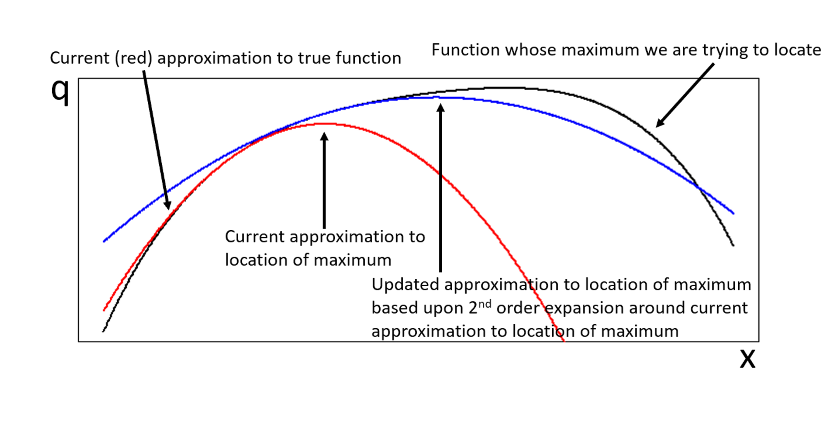
Consider a 1-dimensional example. Let $q(x)$ be the function whose maximum, $x_{*}$ , we are trying to locate. If the expansion of $q(x)$ around our current estimate ${\hat x}_{*}$ of $x_{*}$ is,

$q(x) \;=\; q( {\hat x}_{*} )\;+\; ( x - {\hat x}_{*}) q^{(1)}({\hat x}_{*})\;+\; \frac{1}{2}(x- {\hat x}_{*} )^{2}q^{(2)}({\hat x}_{*})\;+\; O\left ( (x-{\hat x}_{*})^{3}\right )$

The updated estimate of $x_{*}$ is then determined by maximizing the second order expansion above, and is given by,

${\hat x}_{*} \rightarrow {\hat x}_{*} \;-\; \frac{q^{(1)}( {\hat x}_{*})}{q^{(2)}( {\hat x}_{*})}$

The schematic below depicts how the iterative Newton-Raphson procedure locates the maximum of a one-dimensional function.

The multi-dimensional equivalent update rule when we are maximizing a function $q({\boldsymbol x})$ of a vector ${\boldsymbol x}$ is,

$\hat{\boldsymbol x}_{*} \rightarrow \hat{\boldsymbol x}_{*} \;-\; {\boldsymbol H}^{-1}( \hat{\boldsymbol x}_{*})\,\nabla q (\hat {\boldsymbol x}_{*} )\;\;,$

where ${\boldsymbol H}( \hat{\boldsymbol x}_{*})$ is the Hessian of $q({\boldsymbol x})$ evaluated at $\hat{\boldsymbol x}_{*}\;\;.$

As Seeger et al are marginalizing the posterior over $\epsilon_{1}, \epsilon_{2},\ldots,\epsilon_{T-1}, {\boldsymbol l}_{0}$ , the Taylor expansion around any point is necessarily multi-variate, and so ordinarily, finding the maximum of that second order approximation would involve inverting the Hessian of the log-posterior evaluated at the current estimate of the mode. As the latent variables we are trying to marginalize over by doing the Laplace approximation are the $T-1$ innovations, $\epsilon_{1},\;\ldots\;, \epsilon_{T-1}$ and ${\boldsymbol l}_{0}$ , this means that each step of the Newton-Raphson procedure would involve the inversion of a $T\times T$ matrix, i.e. an $O\left(T^{3}\right)$ operation for each Newton-Raphson step. However, Seeger et al point out that once we have replaced the log-posterior by a second-order approximation, finding the maximum of that approximation is equivalent to finding the posterior mean of a linear-Gaussian state-space model, and this can be done using Kalman smoothing. This means in each Newton-Raphson step we need only run a Kalman filter calculation, an $O\left( T \right)$ calculation, rather than a Hessian inversion calculation which would be $O\left(T^{3}\right)$ . When training on, say, 2 years of daily sales data with $T=730$, the speed-up will be significant. Seeger et al do point out that this trick of reducing the computation to one that scales linearly in $T$ is already known within the statistics literature⁴, but not widely known within machine learning.

Seeger et al apply their methodology to a number of real-world scale datasets, for example to a ~40K item dataset with almost a year of historical data at the day-level. Overall run-times for the parameter learning are impressive (typically a few seconds for each of the separate demand model stages), though admittedly this is when running on a 150 node Spark cluster.

References

Working, H. (1943) Statistical laws of family expenditure. J. Am. Statist. Ass., 38:43–56.
Leser, C. E. V. (1963) Forms of Engel functions. Econometrica, 31, 694–703.
Snyder, R., Ord, J., and Beaumont, A. (2012), Forecasting the intermittent demand for slow-moving inventories: A modelling approach. International Journal on Forecasting, 28:485-496
Durbin, J. and Koopman, S. (2012), Time Series Analysis by State Space Methods. Oxford Statistical Sciences. Oxford University Press, 2nd Edition.

Hoyle Analytics

Category: Demand Forecasting

The Past, The Future and The Infrequent: Four books on forecasting

The Books

What the books are about

Demand Forecasting at Amazon

References

The Books

What the books are about

Share this:

References

Share this: