Unsurprisingly, given my day job, I ended up reading several books about forecasting in 2023. On reflection, what was more surprising to me was the variety. The four books I have read (admittedly, not all of them cover-to-cover) span the range from a history of general technology forecasting, the current state of the art and near future of forecasting methods in business, right through to the specific topic of intermittent demand modelling. Hence the title of this blogpost, “The past, the future, and the infrequent”, which is a play on the spaghetti western “The Good, The Bad, and The Ugly”. It also gives me an opportunity to play around with my Stability AI prompting skills to create the headline image above.
The Books
Since I really enjoyed all four of the books, I thought I’d post a short summary and review of each of them. The four books are,
What the books are about
(Top left) – “A History of the Future: Prophets of Progress from H.G. Wells to Isaac Asimov”, by Peter J. Bowler. Published by Cambridge University Press, 2017. ISBN 978-1-316-60262-1.
This is not really a book about forecasting in the way that a Data Scientist would use the word “forecasting”. It is a book about the history of “futurology” – the practice of making predictions about what the world and society will be like in the future, how it will be shaped by technological innovations, and what new technological innovations might emerge. The book reviews the successes and failures of futurologists from the 20th century and what themes were present in those predictions and forecasts. What is interesting is how the forecasts were often shaped by the background and training of the forecaster – forecasts from people with a scientific training or background tended to be more optimistic than those from people with more arts or literary backgrounds. I did read this book from end-to-end.
(Top right) – “Histories of the Future: Milestones in the last 100 years of business forecasting”, by Jonathon P. Karelse. Published by Forbes Books, 2022. ISBN= 978-1-955884-26-6.
This is another book about the history of forecasting. As one of the reviewers, Professor Spyros Makridakis, says on the inside cover of the book, this is not a “how to” guide. However, each chapter of the book does focus on a prominent forecasting method that is used widely in business settings – Chapter 3 covers exponential smoothing, Chapter 5 covers Holt-Winters, Chapter 7 covers Delphi methods – but each method is introduced and discussed from the historical perspective of how the method arose and was used in genuine operational business settings. Consequently, the methods discussed do tend to be the simpler but more robust methods that have stood the test of time of being used in genuine real-world business settings, although the final chapter does discuss AI and ML forecasting methods. This is another book I did read end-to-end.
(Bottom left) – “Demand Forecasting for Executives and Professionals”, by Stephan Kolassa, Bahman Rostami-Tabar, and Enno Siemsen. Published by CRC Press, 2023. ISBN=978-1-032-50772-9.
This is a technical book. However, it has relatively few equations and those equations that it does contain are relatively simple and understandable by anyone with high-school maths, or who has taken a maths module in the first year of a Bachelor’s degree. That is deliberate. As the book says in the preface it “is a high-level introduction to demand forecasting. It will, by itself, not turn you into a forecaster.” The book is aimed at executives and IT professionals whose responsibilities include managing forecasting systems. It is designed to give an overview of the forecasting process as a whole. My only criticism is that, even given the focus on delivering a high-level overview of forecasting and how it should be used and implemented as a process, the topics covered are still ambitious. My experience is that senior managers, even technical ones, won’t have the time to read about ARIMA modelling even at the level it is covered in this book. That said, the breadth of the book (in under 250 pages) and its focus on forecasting as a process is what I like about it. It emphasizes the human element of forecasting via the interaction and involvement that a forecaster or consumer of a forecast has with the forecasting process. These are things you won’t get from a technical book on statistical forecasting methods and that you usually only learn the hard way in practice. If I had an executive or senior IT manager who did want to learn more about forecasting and I could recommend only one book to them, this would be it. As a Data Scientist this is still an interesting book. There is still material I have read and learnt from, but as a Data Scientist it has been a book I have only dipped in and out of.
(Bottom right) – “Intermittent Demand Forecasting: Context, Methods and Application”, by John E. Boylan and Aris A. Syntetos. Published by Wiley 2021. ISBN=978-119-97608-0.
Professor John Boylan passed away in July 2023. I was fortunate enough to attend a webinar in February 2023 that John Boylan gave about intermittent demand forecasting. I learnt a lot from the webinar. It also meant that I was already familiar with a lot of the context on reading the book, making reading the book more enjoyable. In fact, the seminar was where I first came across the book. The book is technical. It is the most technical and focused of the four books reviewed here. It is a book on the best statistical models and methodologies for forecasting intermittent demand, particularly for inventory-management applications. It is an in-depth “how-to” book. As far as I am aware this book is the most up-to-date, comprehensive, and authoritative book on intermittent demand forecasting there is. Since it is a technical book, it is a book I have dipped in and out of, rather than read end-to-end.
I can genuinely recommend all four books. The first two books I enjoyed the most, because I find that personally, reading about the history of how scientific methods and algorithms arise gives extra insight into the nuances of the methods and when and where they work best. The second two books are more “how-to” books – you can find similar material on the internet, in various blog articles and academic papers etc. However, it is always great to have methods explained by practitioners who are also experts in those methods.
The content of the last three books would be more recognizable by your typical working Data Scientist. The first book is more of a book for historians, but I enjoyed it because the subject matter it addressed was in an area/domain relevant to me, that of long-range forecasting.
This is the last in my series of posts on forecasting. The posts have focused on the ‘why’ of forecasting and also some of the practicalities of forecasting. This last post is going to be shorter. It is simply some links to forecasting resources that I’ve found useful or think could be useful – books, articles, online tutorials and software, as well as my opinions on which bits you should focus on learning.
Books/Articles
Forecasting: Methods and Applications by Spyros Makridakis, Steven Wheelwright and Rob Hyndman. This was the book that was recommended to me by a colleague when I started in commercial forecasting. Rob Hyndman (one of the authors) says it is out of date, and recommends his later textbook (see next), but I still find it useful.
Forecasting: Principles and Practice by Rob Hyndman and George Athanasopoulos is considered one of the modern bibles on classical forecasting techniques. It is now in its 3rd edition and also available online for free.
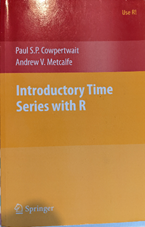
Introductory Time Series with R by Paul Cowpertwait and Andrew Metcalfe. I found this short but concise Springer book (in the Use R! series) on classic time-series analysis in R a great help. It was useful both from an R perspective, but also for short practical introductions and explanations of the various ARIMA concepts. Some of the links to the datasets used are now broken apparently, but I have seen comments that the resources are not hard to find with a google search.
This recent and comprehensive review article in the International Journal of Forecasting is great (arxiv version here). It has short readable paragraphs and sections on a large number of concepts and forecasting topics, so you can simply pick the topic you’re interested in and read just that. Or read the whole article end-to-end if you want.
I’m only going to give links to free open-source software. There are some other excellent commercial applications available, but not everyone will be able to get access to them, so I won’t list them.
R: I have tended to do most of my classical time-series analysis in R. The in-built arima functions and also the forecast package (created by Rob Hyndman and Yeasmin Khandakar) provide a great deal of functionality and are my go-to packages/functions in R for time-series.
The statsmodels package in python provides a similar model building experience to building models in R. Consequently, its time-series functionality provides similar capabilities to that found in R.
Darts package in python: I have done less time-series analysis in python than I have in R. When I have done exploratory time-series analysis in python I have tended to use statsmodels. Having said that, the Darts package, and the Kats package (from Facebook) look like useful python packages from the bits I have read.
Prophet package: The Prophet package, from Facebook, is open-sourced, flexible and very powerful. I have tried it for a couple of tasks. Under the hood it is based upon the Stan probabilistic programming language (PPL), which I have used a lot (both in and outside of my main employment). Prophet is fully automated but I would still recommend you have a basic grasp of classical time-series analysis concepts before you use Prophet, to guard against those situations where a fitted model is inappropriate or clearly wrong.
The engineering team at Uber have also released their own forecasting package, Orbit, which performs Bayesian forecasts using various PPLs under the hood (similar to the way the Prophet package uses Stan).
Methods/Concepts/Techniques you should know about
ARIMA: You should definitely become familiar with the classical approaches to time-series analysis, namely ARIMA. The name is a combination of acronyms, and I’ve given a breakdown of the full acronym and what I think are the important aspects to know about.
AR: Auto-Regressive. These are the ‘lag’ terms in the time-series model equation, whereby the response variable value at timepoint t can depend on the value of the response variable at previous time-points. It is important to understand, i) how the value of the lag coefficients affect the long-run mean and variance of the response variable, including how this determines whether a process is stationary or not, ii) how to determine the order of the AR terms, e.g. by looking at a Partial Auto-Correlation Function (PACF) plot, iii) how the AR terms are infinite impulse response (IIR) terms, in contrast to the finite impulse response (FIR) moving average terms.
I: Integrated. This is the concept within ARIMA that most Data Scientists are least familiar with but a very important one, particularly when dealing with quantities that we naturally expect to grow over time, for example by accumulating increments that increase on average. It is important to understand, i) how to run unit-root tests to test for integrated series – beware the difference between Phillips-Perron (PP) and KPSS tests, as the null hypothesis is different between them, ii) Cointegration and spurious regression (spurious correlation) – for which Clive Granger won a Nobel memorial prize in Economics (shared with Robert Engle) in 2003.
MA: Moving Average. These are the ‘error’ terms in the time-series model equation, whereby the response variable value at timepoint t can be affected by the stochastic error not just at t, but at previous timepoints as well. This allows the response variable to be affected by short timescale perturbations of finite duration (hence the classification of the moving average terms as being finite impulse response terms).
Even if you intend to use only neural network approaches to forecasting, or want to use, say, the Prophet package as an AutoML forecasting solution, it is still a good idea to get a good grasp of ARIMA models. Investing some time in getting to grips with the basics of ARIMA and doing some hands-on playing with ARIMA models will pay huge dividends.
Error Correction Models (ECMs). You may never have need to use Error Correction Models, but they are useful for incorporating the transient departures from a long-term equilibrium. I found these University of Oxford summer school lectures notes given by Prof. Robin Best from Binghamton University (SUNY) a very good and accessible introduction to error correction models. The lecture notes also give excellent explanations of the concepts of integration and co-integration in time-series analysis. I used these lecture notes when I was having to develop an ECM for a long-range stress-testing model.
Neural Network and other Machine Learning techniques: Neural networks have been applied to time-series for a long time, but being blunt, until the last 7 years or so they weren’t very good and didn’t outperform the classical time series approaches (in my opinion). In part that was probably because machine learning practitioners tended to view time-series analysis and forecasting as ‘just another prediction problem’, and so the approaches didn’t really take into account the time-series nature of the data, e.g. the auto-regressive structure, the very things that make time-series what they are. Coupled with the fact that the classical time-series analysis approaches have a very solid theoretical underpinning in ARIMA (expressed in terms of the lag or backshift operator), this meant that machine learning approaches didn’t make as many inroads into time-series analysis as they did in other fields. However, with the advent of Deep Learning approaches using Recurrent Neural Networks and LSTM units, machine learning approaches to time-series analysis have really begun to make their mark. Models such as the DeepAR model from Salinas et al are now considered to outperform classical approaches for specific tasks. Hyndman’s book, “Forecasting: Principles and Practice” contains a chapter on machine learning approaches to time-series analysis, but in my opinion it is only very basic. The extensive review article by Petropoulos et al has a section on ‘Data-Driven Methods’ that includes sub-sections on Neural Networks and also Deep Probabilistic Forecasting Models. However, given the comprehensive nature of the whole review article these sub-sections are necessarily short. Other more extensive resources that I have found useful, which also cover the Deep Learning approaches include,
Lina Faik has an excellent and very up-to-date two-part blog-post on DeepAR and other seq2seq based approaches (Part 1 here, Part 2 here – on Medium) .
That is it. I hope you have enjoyed this series of posts on forecasting. As with anything in Data Science, forecasting isn’t a spectator sport. The best way to learn is to download some datasets and start playing. You will make mistakes, but that is how you learn.
This is part 2 of 3 about producing forecasts in real-world situations. Part 1 was more about the ‘what’ of forecasting, and specifically about different forecast horizons and how those different horizons shape how you do the forecast and what you can do with it. Part 2 is advice to help you avoid common mistakes when producing a forecast.
There are multiple distinct stages to producing and using a forecast. At the simplest level, we can list these different stages as,
Planning a forecast.
Executing a forecast.
Assessing a forecast.
Taking actions or decisions informed by a forecast.
Updating a forecast.
Deploying a forecasting process.
I have found that overwhelmingly the majority of mistakes I’ve made or seen made, are in the planning stage of producing a forecast. In fact, mistakes that I’ve seen in many of the later stages can ultimately be traced back to a failure to plan appropriately. That is, mistakes were made and spotted in one of the later stages, but if we’d thought about it properly, we could have anticipated that the error or issue would occur due to the way the forecasting process had been planned. This introduces our main takeaway,
Put a lot more time and effort into planning the forecasting process than you were initially going to do
</TL;DR>
Let’s get started. Since the majority of errors I’ve seen (and therefore opportunities for learning) are in the planning stage, that is where I’m going to focus most of my discussion. In fact, I am going to simplify the 6 stages outlined to above to just 3 broad areas of discussion,
Mistakes to avoid when planning a forecast
Mistakes to avoid when executing a forecast
Mistakes to avoid when assessing a forecast
In each of those broad areas I’ll introduce a couple of common issues or mistakes that tend to get made, and also provide some hints on how to solve the issues or avoid the mistakes – the issues and solutions will be underlined to highlight them. I’ll also drop in a couple of real-world examples where I’ve seen these mistakes made, or where I made them myself.
Planning
Model Scope:
Issue: The initial information supplied to you is never sufficient to perform an appropriate forecast. This is an unwritten first rule of forecasting1.
There will always be important/crucial things the person requesting the forecast has not told you – out of ignorance or absent-mindedness. This is the time to ask those extra questions, such as,
Why do you need the forecast? What problem are you actually trying to solve? More importantly, what decision are you trying to make using the information the forecast will give?
How are you going to consume the forecast? Is it for insight – identifying the drivers that have the biggest impact on a medium-range outcome? Or is it for strategic planning? Or is it to be incorporated into a machine learning pipeline with an action automatically determined from the result of the forecast, e.g. changing an offer to a segment of customers.
What is the forecast horizon over which you need the forecast?
At what level of time granularity and segmentation do you need the forecast?
Solution: The answers to a) – d) above are inter-related, i.e. the answer to one may uniquely determine the answer to one of the others, but you should still ask each of those questions individually.
By understanding the scope of a system and how the forecast output is actually going to be used we avoid errors such as, failing to identify when the use-case does not justify the time and effort to develop the proposed forecasting model. A good example of this I’ve seen was a model developed for a national social housing charity that needed to predict the future costs of repairs to its housing stock. Due to various operational sensitivities, actions off the back of this prediction could only be taken at the regional level – the charity only needed to predict what the next month’s total repairs costs would be for each region in the country. But …the solution that was built used xgboost to predict the likely repair costs for each house in a region, given details about each house, and then simply aggregated the total predictions to regional level. Over the time horizons being forecasted the housing stock in each region was stable, so an equally accurate forecast could be obtained by using just the actual historical total monthly repair costs. As the historical total monthly repair costs just displayed seasonality and trend, a simple piece of SQL gave a prediction as accurate on a holdout sample as the xgboost based model.
Model Inputs:
Issue: Will you actually know all the input values and model parameter values at forecast time? Check that the values of all the exogenous variables will be known ahead of running the main forecasting model. If the exogenous variables you’ve used in your model include macro-economic quantities, their future values will not be known and you will either need a separate forecasting model for these, or their values will need to be part of the forecast scenario specification. This may be what you intended all along, but you’d be surprised how often someone builds a forecasting model and only afterwards realizes the challenges in specifying the input variables.
This problem can occur even in seemingly benign situations. For example, one mistake I’ve made in the past is using a set of dummy variables to model cohort fixed effects for a model of default rates in a loans portfolio. The only problem was that the loan book was still open – new cohorts were still coming onto the loan book – so to forecast the future default rate of the portfolio required assigning fixed effects to future, as yet unobserved, cohorts. In this instance we chose to make assignment of the future cohort effects part of the scenario specification – scenarios designated future cohorts as ‘high risk’, ‘medium risk’ or ‘low risk’ with the effects values being calculated from an appropriate centile of the historic cohort effects estimates. An alternative approach might have been to treat the cohort effects as random effects and when forecasting marginalize over the random effects of future cohorts. However, the two takeaways from this are, i) when planning a forecast model, think ahead to when you’re going to use it to produce the forecast and make sure you know how you’re going to obtain the input variables, ii) be cautious about including fixed cohort effects when producing forecasts for a changing cohort mix.
Solution: Mentally run through the forecasting process in your head, or on paper, before you start estimating your models. This will flush out issues with the model form or forecasting technique before you have committed to building them.
Issue: Variables/features not included in the model in a sensible or correct form.
I’ve a seen a model built by a marketing team that predicted the response to marketing activity. It was suspected that weather had an impact on how effective the marketing was. This was not an unreasonable hypothesis – when the summer weather is hot and sunny (not that common in the UK) most people want to be outside, in the park or at the beach, not paying close attention to some TV advert. The only problem was that ‘weather’ had been included in the predictive model as the average monthly temperature across the whole of England. There are so many things wrong with this,
The temperature in England on a single day can vary hugely from one place to another. It can be sunny and 25°C in London whilst it is raining and 15°C in Manchester and hailing and 10°C in Newcastle. The England-wide average is a meaningless feature to try and reflect how likely anybody in a specific geography is to respond to marketing. The people in London will be relaxing in the park, ignoring the TV adverts, whilst people in Newcastle will be putting an extra jumper on and hunkering down in front of soap re-runs on the TV.
In a similar vein, the use of a monthly average temperature is pointless. It was believed that the impact of weather on the marketing effectiveness was because of un-seasonal sunny weather over a few days. A monthly average will not reflect this. The monthly England-wide average temperature will reflect just seasonal patterns, not the particular effect the stakeholder was trying to understand.
Temperature is the wrong feature to use here. Hours of sunlight may be better, since the hypothesis was that it was the un-expected very sunny summer weather that was reducing the effectiveness of the marketing. Even better, a feature that captured the presence of unusually hot, dry weather on summer days would be preferable to include in the model. Note that we have now moved from discussing temperature to talking about ‘dry’ summer days, i.e., the absence of any precipitation. When including weather effects in a model it can even be crucial to think what form of precipitation is relevant here. A former colleague told me about some work he’d done for a British mobile phone operator. The mobile company was interested in the impact of weather as they’d noticed that call volumes increased sometimes when there was precipitation. The analysis revealed that, yes, precipitation had an impact, but the form of the precipitation is hugely important. If it’s raining the impact is small, but lower the temperature so that the precipitation comes in the form of snow and the call volumes spike – everybody is phoning home or phoning work to say they are delayed because of snow-blocked roads or trains not running because of ice and snow on the rails. The lesson here is that the precise way in which weather affects our outcome of interest needs to be understood.
Lastly, weather is a prime example of a variable that we won’t automatically know when it comes to producing the forecast. We may have a brilliant forecasting model, but we need to forecast the specific weather feature as well and we may not be able to do that accurately enough to get the benefit of our main forecasting model.
It was suspected that the person who built the model I’ve described just threw ‘weather’ into the model because they were told to. They simply got hold of the easiest or most accessible single weather variable they could find.
Solution: Spend time thinking through the form or particular variant of the feature you are putting into your forecasting model. Will it actually be capable of reflecting the actual effect you are trying to capture in your model? Is it at the right temporal and spatial granularity to be able to do that?
Issue: Insufficient length of training data. Make sure the length of historical data you use to build your forecasting model is sufficiently long. How long is ‘sufficiently long’? Paul Saffo in this 2007 Harvard Business Review article on the 6 Rules For Effective Forecasting says that you should “look back twice as far as you look forward”. I would say you should look back even further. The point here, however, is not to give a precise rule for how much historical data you need for a given forecast horizon, but more to emphasize that the length of historical data you should use is always longer than you think. It should be sufficiently long enough to display several examples of the phenomena you need to capture with your model. To give an example – if you are modelling the effects of macro-economic climate on a financial metric, e.g., loan default rates, then you will want to include several business cycles and more importantly several recessionary periods in your historical training data. How far back in history is still a matter of subjective judgement – for example, was the recession resulting from the 2008 financial crash typical or atypical of the dynamics you want to model and forecast? This highlights two points, i) how far you go back in history can require a detailed discussion and review of the historical data – it is not simply, ‘let’s just include the last two recessions’, ii) you need to have a good idea of what sort of phenomena and/or dynamics you need to model for your forecasts to be representative of the scenarios you are trying to understand. Use the wrong data and the usefulness of your forecasting model may be short-lived. For long-range forecasts you’ll never really know in advance the full range of phenomena that your model needs to capture, as unpredictable and impactful phenomena are always capable of arising within the forecast horizon of a long-range forecast – what are called ‘Black-Swan’ events in parts of the popular science literature. In Part 1 we explained that by considering a very wide range of scenarios we mitigate against this, to a degree. But it means that a model used for long-range forecasting has to have captured dynamics and behaviour appropriate to a very wide range of phenomena – and that can require an awful lot of historical data. Anecdotally, I’ve seen that the length of training data required increases super-linearly with the length of the forecast horizon.
Solution: Think about the kind of phenomena or scenarios you want your model to be capable of forecasting. Does your training data contain adequate examples of such phenomena or scenarios? If yes, then you probably have enough training data. If no, then get additional appropriate training data, or shorten your forecast horizon (see Part I for why you should do this).
Model Form:
Issue: Using a complex or unusual generative modelling technique and believing you can just include the predictive features into the ‘model’ as you would when building a linear model or GLM.
I have seen an agent-based model used to attempt to forecast and identify emergent phenomena that it was believed would occur in response to a macro-economic change or shock. The agent-based simulation was used to mimic the microscopic interactions between the agents and their external environment – the general economy. A macro-economic variable, I think it was unemployment rate, was directly coupled to each agent’s propensity to spend. Lo-and-behold, when the unemployment rate increased the forecast showed that the total expenditure in the system went down. This was hailed as a new finding, showing emergent behaviour. No! It just reflected how the macro-economic variables had been included in the modelling. At this point over 12 months (at 3 FTE, I believe) had been expended on this project.
How the exogenous influences are coupled to a forecasting technique is critically important if we want to identify genuine emergent phenomena. Genuinely emergent phenomena are typically a global property of the system, often resulting from a global constraint. For example, in a physical system it could be a requirement to minimize the overall free energy of the system. In a financial system it could be a requirement to maximize total profit. Ideally, we should think about how the exogenous influences interact with these global constraints when including the exogenous variables in our modelling. If instead the exogenous variables are coupled directly to a metric we will later measure, we should not be surprised when that metric changes when the exogenous variables do.
Solution: The more complex the technique used you more you’ll need to think about how you put the predictive features into the ‘model’.
Issue: Computational optimization of forecast model outputs will exploit the weaknesses in your model. Be aware of the potential future downstream uses of your forecasting process. The forecasting technique you’ve used may not be robust enough to support likely (and anticipatable) downstream uses. It is likely, you’ve set up your forecasting process as an automatable, reproducible codebase. That codebase can then be included in a downstream automated process, such as finding the optimal value of one the actionable input variables. The optimization process will optimize the output of the forecasting model and because forecasts are, almost by definition, ‘out-of-sample’, there is the potential for the optimization process to drive the model to a region of the input space where the model output is non-sensical. This is because the optimization process does not know any better – we have not ensured that the forecasting model output has sensible and credible behaviour for all scenarios or for all sets of input values. To do this we need to build sensible structural constraints or principles into our forecasting model. Such constraints or principles usually come from domain knowledge, e.g. from economic principles when building forecasting models that include macro-economic inputs. These constraints or principles represent assumptions – we are assuming that our system of interest will or should obey classical economic principles. If those assumptions are incorrect, we will be guilty of produced a biased forecast. How do we know when to include such constraints or principles? We don’t know precisely, but we can think before constructing the forecasting model whether the benefits of including them outweigh the dis-advantages, and we are forewarned as to the potential bias. The main point here is, again, think and plan.
Solution: Understand if you will always be in control of the uses of your model. If not, then think whether your model needs to be robust to use-cases you can’t control.
Model Estimation:
Issue: The model estimation process is not set up to reflect what you’re actually trying to model. Use a cost-function that reflects the outcome you care about. When fitting a forecasting model, we will typically be minimizing some cost-function. Choose the cost-function appropriately. If forecast accuracy is going to be assessed using a different cost-function you may want to rethink the cost-function you use for fitting. Or in simple terms, fit your model to optimize the outcome you actually care about.
Solution: Think through each step of the proposed estimation process. Is it ideal for the thing you’re trying to capture.
Execution
Issue: How do you gauge whether your forecast is credible? Always run a baseline calculation or baseline scenario. For a short-range forecast you may have characterized very precisely the scenario you wish to predict, but your baseline scenario can still be something like a Business-As-Usual (BAU) scenario. For long-range forecasting, you can also use a BAU scenario as your baseline scenario but the definition of BAU may be more subjective and contain significant movement in exogenous influences – although it probably won’t be what you consider to be the most extreme scenario. The main benefit of running a baseline scenario is that it allows you to compute realistic ‘deltas’ even if there are far-from-perfect assumptions in your forecasting methodology. Remember the quote from George Box – ‘All models are wrong, but some are useful.’ The skill as a Data Scientist/Statistician is in knowing how to extract the useful insight and information from a ‘wrong’ model. With a baseline calculation you can compute how much worse or better the outcome is under scenario X compared to the baseline scenario. As a human you may then have a feel for what is incorrect in the baseline calculation and correct it or down-weight it. The model based estimate of the delta between scenario X and baseline scenario can then be applied to the human corrected baseline.
Solution: Running a baseline scenario where you have a more intuitive feel for how the system responds will help you assess any other scenario.
Issue: We have a forecast but not a quantitative measure of how confident we are with it. Always produce measures of uncertainty, e.g. confidence intervals for your forecasts. There is limited value in just a point estimate. How sensitive is that estimate to the stochastic component of the response variable dynamics? Then on top that we have uncertainty in the forecast due to parameter uncertainty and potentially also input uncertainty. Sensitivity analysis can help us quantify the impact on the forecast from both parameter uncertainty and input uncertainty, so that we can identify which we need to improve most. Don’t assume that just because values of exogenous variables have been specified for the forecast scenario that they are accurate. Forecast scenarios that are, upfront, specified very precisely can still be mis-specified or specified inappropriately, or even subject to change – it is not unusual for a company to execute a different BAU scenario to what they said they would at the time the forecast was produced.
Solution: Quantify the impact on a forecast from all the major sources of uncertainty. Doing so is essential for framing and qualifying any decisions or actions taken on the back of the forecast output.
Issue: Distinguishing outputs from different forecasts gets messy when you have lots of them. Create a system for time-stamping forecast outputs, the associated input data and meta-data and also the codebase used to produce the forecast. This creates a disciplined process for running, re-running, and changing forecasts whilst knowing which run produced which forecast. You’ll be surprised how often you’ll end up asking yourself questions similar to , ‘now, did I include 5 or 6 years of training data and was it a 2month gap between the end of the training data and the beginning of the forecast horizon?’ Set-up a system to accurately capture what each forecast used, did, and what it was about.
Solution: Set up a system from the outset for timestamping and logging your forecast outputs along with the details on the inputs.
Assessment
Issue: How do you assess the accuracy of your forecasting method if the inputs may also be uncertain? If your forecasting model includes an input feature that itself is forecasted, then always perform holdout tests on your model with and without perfect hindsight.
Testing with perfect hindsight is when we perform the holdout test using the actual observed values of all the input features.
Testing without perfect hindsight is when we perform the holdout test using the forecasted values of any input features that need to be forecasted when actually running in production.
The clear value of performing the two different versions of the holdout tests is that it helps identify where the biggest bottleneck in forecast accuracy is. There is no point in trying to further improve a main forecasting model that is already accurate, say over a 1 year time horizon, if it is only accurate if we know all the inputs precisely and our forecasts of one of the input features is woeful – put the effort into improving the feature forecasting model.
Solution: Assess holdout forecast accuracy with and without perfect hindsight on the input variables.
Issue: How do know whether your complex forecasting technique is adding any value? Always run a baseline technique when assessing holdout accuracy. This is true of any use of machine learning. When building predictive classification models we often build a simple classifier, such as a naïve Bayes classifier, to provide a baseline against which to judge our more complex and sophisticated models and to check that the extra complexity is warranted. Similarly, when producing a forecast for a scenario using our chosen forecasting technique, we should include the forecast from a much simpler technique, such as exponential smoothing. In fact, this commentary, in the International Journal of Forecasting, on the recent M5 forecasting competition suggests 92.5% of the time you won’t beat a simple exponential smoothing model.
Solution: Include a simple baseline forecasting technique.
Issue: Over confidence in the forecast output.
Another of my favourite quotes from the famous statistician George Box,
‘Statisticians, like artists, have the bad habit of falling in love with their models.
George Box
I have been guilty of this myself. We become blind to the possibility that the output from a model can still be garbage even when we have provided high-quality input data. We believe that because we have circumvented the ‘garbage-in, garbage-out’ issue we must have a credible forecast because of the elegance and sophistication of the forecasting technique we have used. We have become seduced by the elegance of the forecasting technique. We have forgotten that ‘all models are wrong’. Well, if a model can be wrong, it can be completely and utterly wrong, and we should remember that. The first rule of forecast assessment – always doubt your forecast. Look at the forecast and see if you can explain to yourself why the forecast has that shape given the inputs.
Solution: Always be prepared to doubt and, if necessary, overrule your forecasts.
That’s Part 2. I hope it has been helpful. In Part 3 I’ll list some forecasting learning resources and tools that I’ve found useful.
Footnote 1: I seem to recall seeing this rule written in a blogpost or paper somewhere, but I’m unable to locate it. If anybody is aware of an original source for it, please let me know.
TL;DR: Forecasting is a process, not just a forecasting model. The over-whelming majority of textbooks will teach you how to build a particular type of forecasting model, but not about how, when and where to use a forecasting process. These things are often learnt only through experience. In this series of blog posts I detail what I have learnt about building forecasts and the forecasting process, through 10 years of commercial Data Science roles. The main takeaways – before you build any forecasting models think long and hard about why you need a forecast, what you are going to do with it, at what granularity and over what time horizon is the forecast needed – long-range forecasting is very different from short-range forecasting. You’ll always need some human involvement in the forecasting process even when using automated short-range forecasts, where it is still advisable to include a human oversight step in the decision making process. The longer the range of the forecast, the more human involvement is advisable.
Why forecast?
Almost all my Data Science roles in the commercial sector have been focused on some form of forecasting – from my first role outside of academia, where I was building long-range ‘stress-testing’ models for the UK’s largest retail bank, through building models that predicted the website clicks for AutoTraderUK in response to a TV advertising campaign, to the demand models I build at dunnhumby to forecast demand for the world’s largest grocery retailers. The focus on forecasting is perhaps no surprise. The ultimate use of the models in business is to help optimize some aspect of the business, be it helping determine the correct Tier 1 capital required to underpin the bank’s risk-weighted-assets, or to determine the best mix of TV channels and timings given a TV marketing budget, through to determining the optimal prices for products in a supermarket category. In all these examples it is the future performance of the business that we want to optimize. The use of forecasting models for business optimization is very much at the ‘prescriptive’ end of the Gartner analytics ascendency staircase. Businesses that use Data Science and ML models in this way are attempting to influence the future towards an outcome that is beneficial for them.
Why the need for this series of posts?
Not all businesses do use Data Science and Machine Learning in this way, or are able to, and so are less in control and more subject to the random winds of chance. Businesses that use forecasting models to optimize business operations tend to be both data and analytics mature. Typically, they have been using analytics in this way for a long time. It is not a new endeavour for those businesses. For other businesses that are new to forecasting there will be a temptation to believe that learning to forecast just requires learning the various forecasting techniques. During my various commercial roles I obviously had to learn the technical details of various forecasting techniques – ARIMA, Holt-Winters, etc. BUT….this article is not another introduction to how to use those various techniques to build models – there are plenty of excellent textbooks and online educational resources that will show you how to do that better than I can1. Instead, this is a series of blog posts about what I have learnt about forecasting along the way. Things which typically aren’t explained in the technical textbooks or technical online articles. Some of these things I’ve learnt the hard way – by making mistakes. Other things I have learnt after the forecast models have been built – when the real challenges of utilizing the models for the actual use case emerge.
Overall, the focus is on how to use forecasting, not how to build specific forecasting models. It will be on understanding what forecasting can do, where you should use it, what it can’t do, and how to get the best out of the forecasting process. I’m going to break this down into a series of 3 posts,
Part1: What is forecasting? What can forecasting be used for?
Part2: How to organize a forecasting process. What to do and what not to do.
Part3: Links to resources and further reading.
Part 1
What is forecasting?
In this era of machine learning and AI can’t we just regard forecasting as just another form of prediction, and forecasting models should be constructed and interpreted just like any other machine learning model? The answer is no.
Forecasting vs Prediction
The high-level distinction between forecasting and prediction is the temporal element. When we forecast we are extrapolating into the future. When we build a predictive model we are usually interpolating within the training set from which the model has been built.
This also highlights that forecasts acknowledge the inherent element of uncertainty within them. Nate Silver in his book, ‘The Signal and the Noise’ notes that some fields such as seismology strongly emphasize this aspect, distinguishing,
A prediction is a definitive and specific statement about when and where an earthquake will strike…whereas a forecast is a probabilistic statement, usually over a longer timescale.
Nate Silver
Nate Silver states that, ‘The United States Geological Survey’s official position is that earthquakes cannot be predicted. They can, however, be forecasted’ – more details from the USGS here.
The temporal element of forecasting is key. It impacts two important aspects of any forecasting model we construct – i) The nature of the variables used in the forecasting model, ii) The time-horizon over which we forecast and what we can use those forecasts for. Let’s look at those two aspects.
Endogenous vs exogenous factors
The temporal element of forecasting means it naturally involves trying to model and/or understand how a system evolves. The factors that influence that evolution can be internal to the system itself -what we call endogenous factors. These are variables that are determined or created by, or emerge from the system itself. An endogenous variable could be as simple as the lagged response variable itself. Other factors that can influence a system’s evolution are external to the system – what we call exogenous factors – such as the broader macro-economic climate when modelling the short-term dynamics of demand for goods or services in a small geographical region.
Forecast horizon
There are multiple temporal components/dimensions/concepts we may need to consider when building a forecasting model,
The time-period used to train a forecasting model.
The time-period over which the forecasting model is tested.
The temporal granularity at which the forecasts are made, e.g. daily, weekly, monthly, etc.
The time increments we use when advancing training/testing windows during the evaluation of the forecasting model.
The time increments we use that set the frequency of the forecasting process when deployed.
The time gap between when the forecasts are made and the date of the first forecast period, i.e., the gap between when the forecasts are made to when they are used.
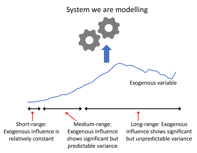
Figure 1: Some of the different temporal concepts involved in defining a forecast.
Some of these concepts are illustrated in Figure 1 above, but perhaps the most important temporal component, and the one I want to focus on, is the length of the forecast horizon – how far into the future are we attempting to forecast? That is, are we making forecasts for the short-term, medium-term, or long-term. The forecast horizon is strongly linked to what a forecast model can be used for (or should be used for), and how it is used. More specifically,
The appropriateness of different forecasting models and techniques is different over the different horizons.
The accuracy of a forecasting model is different over different horizons.
The factors or variables that influence the response variable being forecasted differ over different horizons.
Even how the system being forecasted responds or evolves can be different over different horizons.
The net effect of all this is that the uses of forecasting are and should be different over different forecast horizons. So how do we define the forecast horizon? What defines a short-term horizon, versus a medium-term or long-term horizon? Ultimately, those concepts should be defined in terms of the characteristics or response of the system being forecast, and not the forecasting technique used.
However, there is no universally agreed definition of short-range versus long-range, as this discussion on CrossValidated testifies to. Below I’ll give my own definition and discuss in detail what distinguishes a short-range forecast from a medium-range or long-range forecast. As well as giving a definition based upon the dynamical characteristics of the system being forecasted and the factors that influence it, I’ll also give a second practical definition based upon how we intend to use the forecasts.
Short-range forecasts:
At a trivial level a short-range or short-term forecast is a forecast of the system we are interested in, but over a short period into the future – yes, a very unhelpful definition. So, what precisely defines short-term? It is more helpful to realize that what we mean by ‘short-term’ can vary from system to system. By short-term, we ultimately imply that we expect the behaviour of the system in the immediate past to be reasonable guide to its behaviour in the short-term future – we don’t expect to frequently see massive changes in level of the response variable, and the recent historical values of the response variable alone can enable us to produce a decent forecasting model. We are in the realm where ARIMA models do well. Over a short-term horizon the influence of exogenous variables has not yet begun to kick in, primarily because the important exogenous variables have not changed significantly – they are effectively constant – on these short-term timescales. For a high-street retailer interested in forecasting how many items they will sell, short-term may mean a few days ahead and up to two weeks ahead, whilst for a financial trader involved in ultra-high frequency trading, short-term is measured in milli-seconds and up to only a second or so. For a system whose dynamics are almost entirely endogenous, or systems whose exogenous influences evolve on timescales of years, e.g. climate systems, then short-term can be measured in multiples of years.
The fact that over a short-term horizon any exogenous influences may not vary illustrates that over different forecast horizons the dynamics of our system can be very different. Over short timescales the dynamics is endogenously controlled, over long timescales the dynamics is exogenously controlled.
In complex systems the dynamics over short and long timescales may be different for reasons other than just how the forecast horizon timescale compares to the timescale on which the exogenous influences vary. In complex systems we are likely to have multiple endogenous timescales defined or emergent. This is particularly true for economic systems and we see it in how those systems respond to a shock or a perturbation. Economists have a rule of thumb – in the short-term people are price inelastic (price-insensitive)2, meaning that after a change to a economic system, e.g. supply chain shocks, consumers may not have had time to adapt their behaviour to the new circumstances or the new prices/information available, and so still purchase in a similar manner to before even though prices may have risen. Over longer timescales, people adapt their behaviour – they find cheaper substitutes for the now more expensive item they used to purchase, or they find cheaper suppliers, and so consumers become more price-sensitive again over longer timescales.
The short-term horizon is defined by the shortest timescale process that has an appreciable/relevant influence on the response variable. In our system of interest there may be both exogenous and endogenous processes, and so timescales defined exogenously and endogenously. In a complex system, we will have multiple endogenous timescales, possibly varying by orders of magnitude.
This economic example also highlights that in complex systems and over long timescales we should probably regard everything as ultimately being endogenous due to the degree of inter-connectedness of the various sub-systems. Or in other words, no sub-component of the complex system can be considered on its own as a closed system or independent of other sub-systems, and we should always study the complex system as a whole – but very likely with a lot of simplifying assumptions.
Over the short-term we would expect a forecast to be accurate, or rather capable of being accurate. This doesn’t mean a short-term forecast can’t be massively inaccurate; we could have a extraordinary event and perturbations occur after the the forecast was made, i.e., an assumption that we are forecasting a stable system (a stationary process in statistical language) may turn out to be incorrect due to circumstances that could not have possibly been foreseen – think of a retailer making supply chain forecasts four or six weeks prior to the stock-piling panics that occurred as a consequence of the first Covid-19 lockdowns. Or it may simply be the case that the short-range forecasting model has been poorly built.
Putting unforeseen circumstances and model building competence aside, we would expect a short-range forecast to be reasonably accurate. It can be used for making accurate predictions for very specific scenarios. In contrast, a long-range forecast cannot. This gives us a second practical means of defining forecast horizon. Practically, short-term means the time horizon over which we can use the forecasting model for making detailed specific predictions. Note the emphasis on the word ‘use’. The use-case/business model will define the level of accuracy we require and so can effectively define what is short-range and what is long-range. The recent example of Zillow which exited from US house price forecasting is a case point – see here, here, and here for more detailed discussions. Zillow was using forecasting models over time horizons for which the accuracy was not sufficient to support the particular business model. Zillow was effectively relying on long-range forecasts for detailed predictions, even though the time horizon of 6months ahead may have appeared to be short-term.
The Zillow example illustrates again the difficulty in forecasting complex systems such as markets, particularly if actions taken on the back of the forecast are intended to be part of the market making process. It highlights that perhaps for complex systems we should regards almost all forecasts as long-range.
Medium-range forecasts:
As you might have guessed we can define a medium-term forecast as a forecast over a horizon over which any exogenous influences begin to show significant variation. This is true also for a long-range forecast, but for a medium range forecast horizon we may have a reasonable idea what the values of those exogenous influences may be, or we may even be in control of them, for example they may correspond to actionable variables such as marketing activity variables3. For typical business use-cases medium-range can mean anything from 3-6months out to as much as 18months in the future.
Because exogenous influences start to show significant variation, they can’t simply be absorbed into the intercept of any model, and the typical modelling techniques used are of the form, ‘technique A + X’, meaning that we include the exogenous variables X much like we would when building a standard regression model. Over the medium-term techniques such as ARIMA+X and SARIMA+X are useful.
Long-range forecasts:
By contrast to the definition of what constitutes short-range and medium-range forecasts, a long-range forecast is a forecast over a time-horizon in which exogenous factors have a significant influence and display a significant variance. This could be, for example, macro-economic factors evolving through several business cycles. For the stress-testing models I had to build we were interested in forecasting bank-loan default rates with unemployment rate and central bank base-rate as inputs into the forecasting model. The models were used to produce forecasts with a 5yr forecast horizon. Future unemployment and interest rates were obviously unknown, and so required their own additional forecasting models to predict them.
This macro-economic example highlights that the exogenous influences are themselves subject to variation that is difficult to know in advance. Long-range forecasts have an additional element of uncertainty that increases the final uncertainty of our end forecasts – namely that we probably don’t know all of the inputs to our main forecasting model to a high degree of accuracy. To a large extent this is to be expected. We are forecasting multiple years into the future. In that time many unforeseen circumstances can play-out, e.g., a referendum to leave a major trading block not going the way many people expected, or a global pandemic occurring.
Forecasting exogenous inputs, which encapsulate the influence of national and international contexts, can only be suggestive at best – a reflection of what we think might happen to those exogenous variables, all other things being stable. But….major random, global events do happen. Since we cannot always confidently know what the true future values of the exogenous variable will be, a long-range forecast can only ever be viewed as a ‘what-if’ forecast – what would be the loan default rate if the macro-economic conditions were X. More importantly, a long-range forecast should only ever be used as a ‘what-if’. An individual, specific long-range forecast shouldn’t be used to plan the operation of an organization, or its tactical response to a particular situation.
Does this mean long-range forecasting is useless? No! Far from it! Long-range forecasts won’t tell us what will happen, they tell us what might happen. And so long-range forecasting can be used to help an organization plan strategically. Okay, I hear you say that all forecasts only tell us what might happen, because all forecasts have some uncertainty. What I mean here is that, because the validity of a long-range forecast is dependent on the validity of the input values, we don’t even know if we are looking at an appropriate input scenario. So instead of producing a long-range forecast for a single input scenario, we should always produce a range of long-range forecasts from a range, or ensemble, of input scenarios. The output from an ensemble of long-range forecast then might reveal some behaviours we weren’t expecting, which the business or organization can plan an appropriate response or intervention to. Or alternatively, an ensemble or long-range forecasts may reveal that a particular output metric is largely insensitive to the input scenario, and therefore although we don’t know which scenario will ultimately play-out, we can be confident we know what the value of the metric will be. In our bank stress-testing example we may see that for a wide-ranging ensemble of input scenarios the long-range forecasts indicate that in all the scenarios considered a bank has sufficient capital to withstand the likely increased loan default rates. The bank executives may be confident that no significant capital needs to be raised to protect the bank against whatever the future holds.
You may scoff at last example given financial crisis of 2008, and you may question whether large banks are ever well-prepared for whatever economic future transpires. This may be true, but what it also highlights is that there should always be some discussion around whether the ensemble of input scenarios considered has been wide-ranging enough. Has a big enough stress been applied in the ‘what-if’ scenarios during the stress-testing exercise? This illustrates that long-range forecasting has a high degree of human involvement – to discuss both inputs and interpret outputs. How successful a long-range forecasting exercise is can depend on how an organization approaches it, and how the human contributions/element are brought into play – the excellent non-technical book, Uncharted by Margaret Heffernan discusses these points in depth – I discovered the book through this review by Tim Harford in the Financial Times.
Figure 2: The different forecasting time horizons
Human involvement
The need for significant human involvement in producing some forecasts may be surprising in this era of Data Science and Machine Learning, but direct human involvement in producing forecasts has a long history. Prior to the development of rigorous time series analysis techniques such as ARIMA, this is to be expected. It is interesting to go back and read old articles such as this 1971 Harvard Business Review article on forecasting in business. Putting aside the very gendered language, it is intriguing to see the emphasis upon judgmental forecasting methods and forecasting by analogy. The value of judgmental methods has been re-discovered over the 15 years or so. Specific techniques such as the Delphi method are still widely used in fields as diverse as public transport planning and health. Techniques such as the Delphi method excel at getting a wide range of opinions and inputs to help reduce the uncertainty in understanding complex, many-layered situations. This is what humans are good at. It is also exactly the situation we often face when making long-range forecasts for complex systems. It is unsurprising then that the ability of humans to handle nuanced, ambiguous and complex scenarios is used in other techniques such as prediction markets and superforecasting.
What can we use forecasting for?
The challenges of making long-range forecasts illustrate that there can be markedly different uses of forecasting. Long-range forecasts are about reducing uncertainty through gaining qualitative and semi-quantitative understanding of what might happen. Short-range forecasts are about quantitative prediction of what we think will happen.
There are also other dimensions that differentiate what we can use forecasting for. Three of these that are worth highlighting are,
Insight vs Prediction: This is illustrated well already above by the contrast between short-range forecasts and long-range forecasts, but it is also applicable to short-range or medium-range forecasts on their own. We can use a medium-range forecasting model to make predictions of what will happen in the future, but also to extract insight from the values of the parameters of that model as to what are the relative influences of the different factor upon that future.
Prediction vs Prescription: In my opening paragraphs I highlighted the Gartner analytic ascendency staircase and how some companies have the data and analytic maturity that enable them to use computational forecasting models they’ve built in a prescriptive way – they are used to determine the optimal course of action as opposed to merely forecasting the current baseline scenario.
Different levels of aggregation: When we build any predictive model we have to decide upon the response variable we are going to model. This typically involves a choice about what level of aggregation we going to use – should we build models of individual units (e.g. consumers), groups of units (e.g. a cohort of customers), or the entire population/collection of units (e.g. the entire customer base of an enterprise)? Generally speaking, we should model at the lowest level of granularity at which we first expect to see a homogenous response over the time-horizon of the forecasting exercise. Think of the example of modelling the future default rate of a loans portfolio; if the portfolio is made up of a heterogenous mix of different customer (loan) segments whose response to economic conditions differs across the segments, then as we change the segment mix of that portfolio we will get very different forecast. Modelling the default rate of each homogenous segment separately will allow us to flex that segment mix when exploring different forecast scenarios, whilst modelling the default rate of the portfolio in a single model will not.
Summary:
Forecasting involves extrapolation into the future. This makes it different to other predictive models you might build – these typically involve interpolation within a training dataset. The granularity at which you model is important. Even more important is the horizon over which you are forecasting. A long-term forecast should only be used for exploring behaviour under a range of hypothetical scenarios, whilst short-term and medium-term forecasts can be used to make detailed predictions about specific and highly likely scenarios. Long-range forecasts inform strategic planning, short and medium-term forecast inform tactical responses. This means that when forecasting we should identify what kind of forecast we want and onlythen choose our forecasting technique appropriately.
In the next part of this series of blog posts I will cover some of the do’s and don’ts of forecasting. It won’t be about how to use a particular forecast model building technique. It will be about the common mistakes made – including ones I’ve made or I’ve seen made – so that you can avoid them (in the future).
Footnotes
This very recent review by Petropoulos et al (to appear in International Journal of Forecasting) gives both a comprehensive coverage of the different forecasting techniques available and also a comprehensive set of case studies. The case studies illustrate the practice and challenges of forecasting in individual sectors and so touch in part on some of the issues I’ll be discussing. I’ll also be aiming to give broad general advice (not sector specific) on the practice of forecasting.
See for example, Milgrom, Paul and Roberts, John. “The LeChatelier Principle.” American Economic Review, March 1996, 86(1):173-179.
For the purposes of this blog and for simplicity I’m going to ignore the subtle distinction of whether price and marketing variables in demand models are exogenous or endogenous. I’m going to consider them here as exogenous since they are being imposed or set by the marketer or retailer. However, price drives demand and demand drives the price, so it is common to consider price to be an endogenous variable over longer timescales and within the more complex system consisting jointly of the retailer and the consumer.


 There will always be important/crucial things the person requesting the forecast has not told you – out of ignorance or absent-mindedness. This is the time to ask those extra questions, such as,

 value in just a point estimate. How sensitive is that estimate to the stochastic component of the response variable dynamics? Then on top that we have uncertainty in the forecast due to parameter uncertainty and potentially also input uncertainty. Sensitivity analysis can help us quantify the impact on the forecast from both parameter uncertainty and input uncertainty, so that we can identify which we need to improve most. Don’t assume that just because values of exogenous variables have been specified for the forecast scenario that they are accurate. Forecast scenarios that are, upfront, specified very precisely can still be mis-specified or specified inappropriately, or even subject to change – it is not unusual for a company to execute a different BAU scenario to what they said they would at the time the forecast was produced.