Comparison of Benford's Law and the proportion of first digits from file sizes of files on my laptop hard drive.

A Christmas Cracker Puzzle – Part 2

On January 19, 2025May 26, 2025 By dchoyleIn Data Science, Fun Mathematics, Miscellaneous, Scientific computation1 Comment

Before Christmas I set a little puzzle. The challenge was to calculate the proportion of file sizes on your hard drive that start with the digit 1. I predicted that the proportion you got was around 30%. I’ll now explain why.

Benford’s Law

The reason why around 30% of all the file sizes on your hard disk start with 1 is because of Benford’s Law. Computer file sizes approximately follow Benford’s Law.

What is Benford’s Law?

Benford’s Law says that for many datasets the first digits of the numbers in the dataset follow a particular distribution. Under Benford’s Law, the probability of the first digit being equal to d is,

$\log_{10} ( 1 + \frac{1}{d} )\;\;\;.\;\;\;\;\;\;$ Eq.1

So, in a dataset that follows Benford’s Law, the probability that a number starts with a 1 is around 30%. Hence, the percentage of file sizes that start with 1 is around 30%.

The figure below shows a comparison of the distribution in Eq.1 and the distribution of first digits of file sizes for files in the “Documents” folder of my hard drive. The code I used to calculate the empirical distribution in the figure is given at the end of this post. You can see the distribution derived from my files is in very close agreement with the distribution predicted by Eq.1. The agreement between the two distributions in the figure is close but not perfect – more on that later.

Benford’s Law is named after Frank Benford, whose discovered the law in 1938 – see the later section for some of the long history of Benford’s Law. Because Benford’s Law is concerned with the distribution of first digits in a dataset, it is also commonly referred to as, ‘the first digit law’ and also the ‘significant digit law’.

Benford’s Law is more than just a mathematical curiosity or Christmas cracker puzzle. It has some genuine applications – see later. It has also fascinated mathematicians and statisticians because it applies to so many diverse datasets. Benford’s Law has been shown to apply to datasets as different as the size of rivers and election results.

What’s behind Benford’s Law

The intuition behind Benford’s Law is that if we think there are no a priori constraints on what value a number can take then we can make the following statements,

We expect the numbers to be uniformly distributed in some sense – more on that in a moment.
There is no a priori scale associated with the distribution of numbers. So, I should be able to re-scale all my numbers and have a distribution with the same properties.

Overall, this means we expect the numbers to be uniformly distributed on a log scale.

This intuition helps us identify when we should expect a dataset to follow Benford’s Law, and it also gives us a hand-waving way of deriving the form of Benford’s Law in Eq.1.

Deriving Benford’s Law

First, we restrict our numbers to be positive and derive Benford’s Law. The fact that Benford’s Law would also apply to negative numbers once we ignore their sign should be clear.

We’ll also have to restrict our positive numbers to lying in some range $[\frac{1}{x_{max}}, x_{max}]$ so that the probability distribution of $x$ is properly normalized. We’ll then take the limit $x_{max}\rightarrow\infty$ at the end. For convenience, well take $x_{max}$ to be of the form $x_{max} = 10^{k_{max}}$ , and so the limit $x_{max}\rightarrow\infty$ corresponds to the limit $k_{max}\rightarrow\infty$ .

Now, if our number $x$ lies in $[\frac{1}{x_{max}}, x_{max}]$ and is uniformly distributed on a log-scale, then the probability density for $x$ is,

$p(x) = \frac{1}{2\ln x_{max}} \frac{1}{x}\;\;.$

The probability of getting a number between, say 1 and 2 is then,

${\rm{Prob}} \left ( 1 \le x < 2 \right ) = \frac{1}{2\ln x_{max}} \int_{1}^{2} \frac{1}{x} dx \;\;.$

Now numbers which start with a digit $d$ are of the form $a10^{k}$ with $a \in [d, d+1)$ and $k = -k_{max},\ldots,-2,-1,0,1,2,\ldots,k_{max}$ . So, the total probability of getting such a number is,

${\rm{Prob}} \left ( {\rm{first\;digit}}\;=\;d \right ) = \sum_{k=-k_{max}}^{k_{max}}\frac{1}{2\ln x_{max}}\int_{d10^{k}}^{(d+1)10^{k}} \frac{1}{x} dx\;\; ,$

and so after performing the integration and summation we have,

${\rm{Prob}} \left ( {\rm{first\;digit}}\;=\;d \right ) = \frac{2k_{max}}{2\ln x_{max}} \left [ \ln ( d+1 ) - \ln d\right ]\;\;.$

Recalling that we have chosen $x_{max} =10^{k_{max}}$ , we get,

${\rm{Prob}} \left ( {\rm{first\;digit}}\;=\;d \right ) = \frac{1}{\ln 10} \left [ \ln ( d+1 ) - \ln d\right ]\;=\;\log_{10} \left ( 1 + \frac{1}{d}\right )\;\;.$

Finally, taking the limit $k_{max}\rightarrow\infty$ gives us Benford’s Law for positive valued numbers which are uniformly distributed on a log scale.

Ted Hill’s proof of Benford’s Law

The derivation above is a very loose (lacking formal rigour) derivation of Benford’s Law. Many mathematicians have attempted to construct a broadly applicable and rigorous proof of Benford’s Law, but it was not until 1995 that a widely accepted proof was derived by Ted Hill from Georgia Institute of Technology. You can find Hill’s proof here. Ted Hill’s proof also seemed to reinvigorate interest in Benford’s Law. In the following years there were various popular science articules on Benford’s Law, such as this one from 1999 by Robert Matthews in The New Scientist. This article was where I first learned about Benford’s Law.

Benford’s Law is base invariant

The approximate justification we gave above for why Benford’s Law works made no explicit reference to the fact that we were working with numbers expressed in base 10. Consequently, that justification would be equally valid if we were working with numbers expressed in base $b$ . This means that Benford’s Law is base invariant, and a similar derivation can be made for base $b$ .

The distribution of first digits given in Eq.1 is for numbers expressed in base 10. If we express those same numbers in base $b$ and write a number $x$ in base $b$ as,

$x = x_{1}x_{2}x_{3}\ldots x_{K}\;\;,$

then the first digit $x_{1}$ is in the set $\{1,2,3,\ldots,b-1\}$ and the probability that the first digit has value $d$ is given by,

${\rm{Prob}} \left ( x_{1}\;=\;d \right ) = \log_{b}\left ( 1 + \frac{1}{d}\right )\;\;\;,\; d\in\{1,2,3,\ldots,b-1\}\;\;\;.\;\;\;\;\;$ Eq.2

When should a dataset follow Benford’s Law?

The broad intuition behind Benford’s Law that we outlined above also gives us an intuition about when we should expect Benford’s Law to apply. If we believe the process generating our data is not restricted in the scale of the values that can be produced and there are no particular values that are preferred, then a large dataset drawn from that process will be well approximated by Benford’s Law. These considerations apply to many different types of data generating processes, and so with hindsight it should not come as a surprise to us that many different datasets appear to follow Benford’s Law closely.

This requires that no scale emerges naturally from the data generating process. This means the data values shouldn’t be clustered around a particular value, or particular values. So, data drawn from a Gaussian distribution would not conform to Benford’s law. From the perspective of the underlying processes that produce the data, this means there shouldn’t be any equilibrium process at work, as that would drive the measured data values to the value corresponding to the equilibrium state of the system. Likewise, there should be no constraints on the system generating the data, as the constraints will drive the data towards a specific range of values.

However, no real system is truly scale-free. The finite system size always imposes a scale. However, if we have data that can vary over many orders of magnitude then from a practical point of view, we can regard that data as effectively scale free. I have found that data that varies over 5 orders of magnitude is usually well approximated by Benford’s law.

Because a real-world system cannot really ever truly satisfy the conditions for Benford’s Law, we should expect that most real-world datasets will only show an approximate agreement with Benford’s Law. The agreement can be very close, but we should still expect to see deviations from Benford’s Law – just as we saw in the figure at the top of this post. Since real-world datasets won’t follow Benford’s Law precisely, we also shouldn’t expect to see a real-world dataset follow the base-invariant form of Benford’s Law in Eq.2 for every choice of base. In practice, this means that there is usually a particular base $b$ for which we will see closer agreement with the distribution in Eq.2, compared to other choices of base.

Why computer file sizes follow Benford’s Law

Why does Benford’s Law apply to the sizes of the files on your computer? Those file sizes can span over several orders of magnitude – from a few hundred bytes to several hundred megabytes. There is also no reason why my files should cluster around a particular file size – I have photos, scientific and technical papers, videos, small memos, slides, and so on. It would be very unusual if all those different types of files, from different use cases, end up having very similar sizes. So, I expect Benford’s Law to be a reasonable description of the distribution of first digits of the file sizes of files in my “Documents” folder.

However, if the folder I was looking at just contained, say, daily server logs, from a server that ran very unexciting applications, I would expect the server log file size to be very similar from one day to the next. I would not expect Benford’s Law to be a good fit to those server log file sizes.

In fact a significant deviation from Benford’s Law in the file size distribution would indicate that we have a file size generation process that is very different from a normal human user going about their normal business. That may be entirely innocent, or it could be indicative of some fraudulent activity. In fact, fraud detection is one of the practical applications of Benford’s Law.

The history of Benford’s Law

Simon Newcomb

One of the reasons why the fascination with Benford’s Law endures is the story of how it was discovered. With such an intriguing mathematical pattern, it is perhaps no surprise to learn that Frank Benford was not the first scientist to spot the first-digit pattern. The astronomer Simon Newcomb had also published a paper on, “the frequency of use of the different digits in natural numbers” in 1881. Before the advent of modern computers, scientists and mathematicians computed logarithms by looking them up in mathematical tables – literally books of logarithm values. I still have such a book from when I was in high-school. The story goes that Newcomb noticed that in a book of logarithms the pages were grubbier, i.e. used more, for numbers whose first significant digit was 1. From this Newcomb inferred that numbers whose first significant digit was 1 must be more common, and he supposedly even inferred the approximate frequency of such numbers from the relative grubbiness of the pages in the book of logarithms.

In more recent years the first-digit law is also referred to as the Newcomb-Benford Law, although Benford’s Law is still more commonly used because of Frank Benford’s work in popularizing it.

Benford’s discovery

Frank Benford rediscovered the law in 1938, but also showed that data from many diverse datasets – from the surface area of rivers to population sizes of US counties – appeared to follow the distribution in Eq.1. Benford then published his now famous paper, “The law of anomalous numbers”.

Applications of Benford’s Law

There are several books on Benford’s Law. One of the most recent, and perhaps the most comprehensive is Benford’s Law: Theory and Applications. It is divided into 2 sections on General Theory (a total of 6 chapters) and 4 sections on Applications (a total of 13 chapters). Those applications cover the following:

Detection of accounting fraud
Detection of voter fraud
Measurement of the quality of economic statistics
Uses of Benford’s Law in the natural sciences, clinical sciences, and psychology.
Uses of Benford’s Law in image analysis.

I like the book because it has extensive chapters on applications written by practitioners and experts on the uses of Benford’s Law, but the application chapters make links back to the theory.

Many of the applications, such as fraud detection, are based on the idea of detecting deviations from the Benford Law distribution in Eq.1. If we have data that we expect to span several orders of magnitude and we have no reasons to suspect the data values should naturally cluster around a particular value, then we might expect it to follow Benford’s Law closely. This could be sales receipts from a business that has clients of very different sizes and sells goods or services that vary over a wide range of values. Any large deviation from Benford’s Law in the sales recipts would then indicate the presence of a process that produces very specific receipt values. That process could be data fabrication, i.e. fraud. Note, this doesn’t prove the data has been fraudulently produced, it just means that the data has been produced by a process we wouldn’t necessarily expect.

My involvement with Benford’s Law

In 2001 I published a paper demonstrating that data from high-throughput gene expression experiments tended to follow Benford’s Law. The reasons why mRNA levels should follow Benford’s Law is ultimately those we have already outlined – mRNA levels can range over many orders of magnitude and there are no a priori molecular biology reasons why, across the whole genome, mRNA levels should be centered around a particular value.

In December 2007 a conference on Benford’s Law was organized by Prof. Steven Miller from Brown University and others. The conference was held in a hotel in Sante Fe and was sponsored/funded by Brown University, the University of New Mexico, Universidade de Vigo, and the IEEE. Because of my 2001 paper, I received an invitation to talk at the workshop.

For me, the workshop was very memorable for many reasons,

I had a very bad cold at the time.
Due to snow in both the UK and US, I was snowbound overnight in Chicago airport (sleeping in the airport), and only just made a connecting flight in Dallas to Albuquerque. Unfortunately, my luggage didn’t make the flight connection and ended up getting lost in all the flight re-arrangements and didn’t show up in Santa Fe until 2 days later.
It was the first time I’d seen snow in the desert – this really surprised me. I don’t know why, it just did.
Because of my cold, I hadn’t finished writing my presentation. So I stayed up late the night before my talk to finish writing my slides. To sustain my energy levels through the night whilst I was finishing writing my slides, I bought a Hershey bar thinking it would be similar to chocolate bars in the UK. I took a big bite from the Hershey bar. Never again.
But this was all made up for by the fact I got to sit next to Ted Hill during the workshop dinner. Ted was one of the most genuine and humble scientists I have had the pleasure of talking to. Secondly, the red wine at the workshop dinner was superb.

From that workshop Steven Miller organized and edited the book on Benford’s Law I referenced above. Hence why I think that book is one of the best on Benford’s Law, although I am biased as I contributed one of the chapters – Chapter 16 on “Benford’s Law in the Natural Sciences”

My Python code solution

To end this post, I have given below the code I used to calculate the distribution of first digits of the file sizes on my laptop hard drive.

import numpy as np

# We'll use the pathlib library to recurse over
# directories
from pathlib import Path

# Specify the top level directory
start_dir = "C:\\Users\\David\\Documents"

# Use a list comprehension to recursively loop over all sub-directories 
# and get the file sizes
filesizes = [path.lstat().st_size for path in list(Path(start_dir).glob('**/*' )) if path.is_file()]

# Now count how many file sizes start with a 1
proportion1 = np.sum([int(str(i)[0])==1 for i in filesizes])/len(filesizes)

# Print the result
print("Proportion of filesizes starting with 1 = " + str(proportion1))
print("Number of files = " + str(len(filesizes)))

# Calculate the first-digit proportions for all digits 1 to 9
proportions = np.zeros(9)
for i in range(len(filesizes)):
    proportions[int(str(filesizes[i])[0])-1] += 1.0 
    
proportions /= len(filesizes)

A Christmas Cracker Puzzle – Part 1

On December 17, 2024January 19, 2025 By dchoyleIn Fun Mathematics, Mathematical Analysis, Miscellaneous1 Comment

Here’s an interesting little coding challenge for you, with a curious data twist at the end. Less of an Advent of Code challenge and more of a Christmas Cracker puzzle.

Without knowing anything about you, I will make a prediction about the size of the files you have on your computer. Christmas magic? Maybe. Read on to find out.

There are two parts to this puzzle

Part 1 – Obtain a list of file sizes (in bytes) of all the files on your computer that are in a high-level directory and its sub-directories. We’re talking here about files with a non-zero file size. We also talking about actual files, so the folders/directories themselves should not be included, just their file contents. If this is your own laptop the high-level directory could be the Documents directory (if on Windows). Obviously, you’ll need to have permission to recurse over all the sub-directories. You should choose a starting directory that has a reasonably large number of files in total across all its sub-directories.

Part 2 – Calculate the proportion of files whose file size starts with a 1. So, if you had 10 files of sizes, 87442, 78922, 3444, 9653, 197643, 26768, 8794787, 22445, 7654, 56573, then the proportion of files whose file size starts with a 1 is 0.1 or 10%.

The overall goal

The goal is to write code that performs the two parts of the challenge in as efficient a way as possible. You can use whatever programming languages you want to perform the two parts – you might use the command line for the first part and a high-level programming language for the second, or you might use a high-level programming language for both parts.

I used Python for both parts and used the Documents directory on my laptop as my starting directory. I had 96351 files in my Documents folder and its sub-directories. The proportion of my files that have a size starting with 1 is approximately 0.31, or 31%.

The twist

Now for the curious part. You should get a similar proportion, that is, around 30%. I will explain why in a separate post (part 2) in the new year, and why if you don’t it can tell us something interesting about the nature of the files on your computer.

You’re going to need a bigger algorithm – Amdahl’s Law and your responsibilities as a Data Scientist

On February 2, 2024December 17, 2024 By dchoyleIn Algorithms, Data Science, Mathematical Analysis, Scientific computationLeave a comment

You have some prototype Data Science code based on an algorithm you have designed. The code needs to be productionized, and so sped up to meet the specified production run-times. If you stick to your existing technology stack, unless the runtimes of your prototype code are within a factor of 1000 of your target production runtimes, you’ll need a bigger, better algorithm. There is a limit to what speed up your technology stack can achieve. Why is this? Read on and I’ll explain. And I’ll explain what you can do if you need more than a 1000-fold speed up of your prototype.

Speeding up your code with your current tech stack

There are two ways in which you can speed up your prototype code,

Improve the efficiency of the language constructs used, e.g. in Python replacing for loops with list comprehensions or maps, refactoring subsections of the code etc.
Horizontal scaling of your current hardware, e.g. adding more nodes to a compute cluster, adding more executors to the pool in a Spark cluster.

Point 2 assumes that your calculation is compute bound and not memory bound, but we’ll stick with that assumption for this article. We also exclude the possibility that the productionization team can invent or buy a new technology that is sufficiently different or better than your current tech stack – it would be an unfair ask of the ML engineers to have to invent a whole new technology just to compensate for your poor prototype. They may be able to to, but we are talking solely about using your current tech stack and we assume that it does have some capacity to be horizontally scaled.

So what speed ups can we expect from points 1 and 2 above? Point 1 is always possible. There are always opportunities for improving code efficiency that you or another person will spot when looking at the code for a second time. A more experienced programmer reviewing the code can definitely help. But let’s assume that you’re a reasonably experienced Data Scientist yourself. It is unlikely that your code is so bad that a review by someone else would speed it up by more than a factor of 10 or so.

So if the most we expect from code efficiency improvements is a factor 10 speed up, what speed up can we additionally get from horizontal scaling of your existing tech stack? A factor of 100 at most. Where does this limit of 100 come from? Amdahl’s law.

Amdahl’s law

Amdahl’s law is a great little law. Its origins are in High Performance Computing (HPC), but it has a very intuitive basis and so is widely applicable. Because of that it is worth explaining in detail.

Imagine we have a task that currently takes time T to run. Part of that task can be divided up and performed by separate workers or resources such as compute nodes. Let’s use P to denote the fraction of the task that can be divided up. We choose the symbol P because this part of the overall task can be parallelized. The fraction that can’t be divided up we denote by S, because it is the non-parallelizable or serial part of the task. The serial part of the task represents things like unavoidable overhead and operations in manipulating input and output data-structures and so on.

Obviously, since we’re talking about fractions of the overall runtime T, the fractions P and S must sum to 1, i.e.

The parallelizable part of the task takes time TP to run, whilst the serial part takes time TS to run.

What happens if we do parallelize that parallelizable component P? We’ll parallelize it using N workers or executors. When N=1, the parallelizable part took time TP to run, so with N workers it should (in an ideal world) take time TP/N to run. Now our overall run time, as a function of N is,

This is Amdahl’s law¹. It looks simple but let’s unpack it in more detail. We can write the speed up factor in going from T(N=1) to T(N) as,

The figure below shows plots of the speed-up factor against N, for different values of S.

From the plot in the figure, you can see that the speed up factor initially looks close to linear in N and then saturates. The speed up at saturation depends on the size of the serial component S. There is clearly a limit to the amount of speed up we can achieve. When N is large, we can approximate the speed up factor in Eq.3 as,

From Eq.4 (or from Eq.3) we can see the limiting speed up factor is 1/S. The mathematical approximation in Eq.4 hides the intuition behind the result. The intuition is this; if the total runtime is,

then at some point we will have made N big enough that P/N is smaller than S. This means we have reduced the runtime of the parallelizable part to below that of the serial part. The largest contribution to the overall runtime is now the serial part, not the parallelizable part. Increasing N further won’t change this. We have hit a point of rapidly diminishing returns. And by definition we can’t reduce S by any horizontal scaling. This means that when P/N becomes comparable to S, there is little point in increasing N further and we have effectively reached the saturation speed up.

How small is S?

This is the million-dollar question, as the size of S determines the limiting speed up factor we can achieve through horizontal scaling. A larger value of S means a smaller speed up factor limit. And here’s the depressing part – you’ll be very lucky to get S close to 1%, which would give you a speed up factor limit of 100.

A real-world example

To explain why S = 0.01 is around the lowest serial fraction you’ll observe in a real calculation, I’ll give you a real example. I first came across Amdahl’s law in 2007/2008, whilst working on a genomics project, processing very high-dimensional data sets². The calculations I was doing were statistical hypothesis tests run multiple times.

This is an example of an “embarrassingly parallel” calculation since it just involves splitting up a dataframe into subsets of rows and sending the subsets to the worker nodes of the cluster. There is no sophistication to how the calculation is parallelized, it is almost embarrassing to do – hence the term “embarrassingly parallel”.

The dataframe I had was already sorted in the appropriate order, so parallelization consisted of taking a small number of rows off the top of dataframe and sending to a worker node and repeating. Mathematically, on paper, we had S=0. Timings of actual calculations with different numbers of compute nodes and fitting an Amdahl’s law curve to those timings revealed we had something between S=0.01 and S=0.05.

A value of S=0.01 gaves us a maximum speed up factor of 100 from horizontal scaling. And this was for a problem that on paper had S=0. In reality, there is always some code overhead in manipulating the data. A more realistic limit on S for an average complexity piece of Data Science code would be S=0.05 or S=0.1, meaning we should expect limits on the speed up factor of between 10 and 20.

What to do?

Disappointing isn’t it!? Horizontal scaling will speed up our calculation by at most a factor of 100, and more likely only a factor of 10-20. What does it mean for productionizing our prototype code? If we also include the improvements in the code efficiency, the most we’re likely to be able to speed up our prototype code by is a factor of 1000 overall. It means that as a Data Scientist you have a responsibility to ensure the runtime of your initial prototype is within a factor of 1000 of the production runtime requirements.

If a speed up of 1000 isn’t enough to hit the production run-time requirements, what can we do? Don’t despair. You have several options. Firstly, you can always change the technology underpinning your tech stack. Despite what I said at the beginning of this post, if you are repeatedly finding that horizontal scaling of your current tech stack does not give you the speed-up you require, then there may be a case for either vertical scaling the runtime performance of each worker node or using a superior tech stack if one exists.

If improvement by vertical scaling of individual compute nodes is not possible, then there are still things you can do to mitigate the situation. Put the coffee on, sharpen your pencil, and start work on designing a faster algorithm. There are two approaches you can use here,

Reduce the performance requirements: This could be lowering the accuracy through approximations that are simpler and quicker to calculate. For example, if your code involves significant matrix inversion operations you may be able to approximate a matrix by its diagonal and explicitly hard code the calculation of its inverse rather than performing expensive numerical inversion of the full matrix.
Construct a better algorithm: There are no easy recipes here. You can get some hints on where to focus your effort and attention by identifying the runtime bottlenecks in your initial prototype. This can be done using code profiling tools. Once a bottleneck has been identified, you can then progress by simplifying the problem and constructing a toy problem that has the same mathematical characteristics as the original bottleneck. By speeding up the toy problem you will learn a lot. You can then apply those learnings, even if only approximately, to the original bottleneck problem.

When I first stumbled across Amdahl’s law, I mentioned it to a colleague working on the same project as I was. They were a full-stack software developer and immediately, said “oh, you mean Amdahl’s law about limits on the speed you can write to disk?”. It turns out there is another Amdahl’s Law, often called “Amdahl’s Second Law”, or “Amdahl’s Other Law”, or “Amdahl’s Lesser Law”, or “Amdahl’s Rule-Of-Thumb”. See this blog post, for example, for more details on Amdahl’s Second Law.
Hoyle et. al, “Shared Genomics: High Performance Computing for distributed insights in genomic medical research”, Studies in Health Technology & Informatics 147:232-241, 2009.

The Past, The Future and The Infrequent: Four books on forecasting

On January 6, 2024February 2, 2024 By dchoyleIn Demand Forecasting, ForecastingLeave a comment

Unsurprisingly, given my day job, I ended up reading several books about forecasting in 2023. On reflection, what was more surprising to me was the variety. The four books I have read (admittedly, not all of them cover-to-cover) span the range from a history of general technology forecasting, the current state of the art and near future of forecasting methods in business, right through to the specific topic of intermittent demand modelling. Hence the title of this blogpost, “The past, the future, and the infrequent”, which is a play on the spaghetti western “The Good, The Bad, and The Ugly”. It also gives me an opportunity to play around with my Stability AI prompting skills to create the headline image above.

The Books

Since I really enjoyed all four of the books, I thought I’d post a short summary and review of each of them. The four books are,

What the books are about

(Top left) – “A History of the Future: Prophets of Progress from H.G. Wells to Isaac Asimov”, by Peter J. Bowler. Published by Cambridge University Press, 2017. ISBN 978-1-316-60262-1.
- This is not really a book about forecasting in the way that a Data Scientist would use the word “forecasting”. It is a book about the history of “futurology” – the practice of making predictions about what the world and society will be like in the future, how it will be shaped by technological innovations, and what new technological innovations might emerge. The book reviews the successes and failures of futurologists from the 20^th century and what themes were present in those predictions and forecasts. What is interesting is how the forecasts were often shaped by the background and training of the forecaster – forecasts from people with a scientific training or background tended to be more optimistic than those from people with more arts or literary backgrounds. I did read this book from end-to-end.
(Top right) – “Histories of the Future: Milestones in the last 100 years of business forecasting”, by Jonathon P. Karelse. Published by Forbes Books, 2022. ISBN= 978-1-955884-26-6.
- This is another book about the history of forecasting. As one of the reviewers, Professor Spyros Makridakis, says on the inside cover of the book, this is not a “how to” guide. However, each chapter of the book does focus on a prominent forecasting method that is used widely in business settings – Chapter 3 covers exponential smoothing, Chapter 5 covers Holt-Winters, Chapter 7 covers Delphi methods – but each method is introduced and discussed from the historical perspective of how the method arose and was used in genuine operational business settings. Consequently, the methods discussed do tend to be the simpler but more robust methods that have stood the test of time of being used in genuine real-world business settings, although the final chapter does discuss AI and ML forecasting methods. This is another book I did read end-to-end.
(Bottom left) – “Demand Forecasting for Executives and Professionals”, by Stephan Kolassa, Bahman Rostami-Tabar, and Enno Siemsen. Published by CRC Press, 2023. ISBN=978-1-032-50772-9.
- This is a technical book. However, it has relatively few equations and those equations that it does contain are relatively simple and understandable by anyone with high-school maths, or who has taken a maths module in the first year of a Bachelor’s degree. That is deliberate. As the book says in the preface it “is a high-level introduction to demand forecasting. It will, by itself, not turn you into a forecaster.” The book is aimed at executives and IT professionals whose responsibilities include managing forecasting systems. It is designed to give an overview of the forecasting process as a whole. My only criticism is that, even given the focus on delivering a high-level overview of forecasting and how it should be used and implemented as a process, the topics covered are still ambitious. My experience is that senior managers, even technical ones, won’t have the time to read about ARIMA modelling even at the level it is covered in this book. That said, the breadth of the book (in under 250 pages) and its focus on forecasting as a process is what I like about it. It emphasizes the human element of forecasting via the interaction and involvement that a forecaster or consumer of a forecast has with the forecasting process. These are things you won’t get from a technical book on statistical forecasting methods and that you usually only learn the hard way in practice. If I had an executive or senior IT manager who did want to learn more about forecasting and I could recommend only one book to them, this would be it. As a Data Scientist this is still an interesting book. There is still material I have read and learnt from, but as a Data Scientist it has been a book I have only dipped in and out of.
(Bottom right) – “Intermittent Demand Forecasting: Context, Methods and Application”, by John E. Boylan and Aris A. Syntetos. Published by Wiley 2021. ISBN=978-119-97608-0.
- Professor John Boylan passed away in July 2023. I was fortunate enough to attend a webinar in February 2023 that John Boylan gave about intermittent demand forecasting. I learnt a lot from the webinar. It also meant that I was already familiar with a lot of the context on reading the book, making reading the book more enjoyable. In fact, the seminar was where I first came across the book. The book is technical. It is the most technical and focused of the four books reviewed here. It is a book on the best statistical models and methodologies for forecasting intermittent demand, particularly for inventory-management applications. It is an in-depth “how-to” book. As far as I am aware this book is the most up-to-date, comprehensive, and authoritative book on intermittent demand forecasting there is. Since it is a technical book, it is a book I have dipped in and out of, rather than read end-to-end.

I can genuinely recommend all four books. The first two books I enjoyed the most, because I find that personally, reading about the history of how scientific methods and algorithms arise gives extra insight into the nuances of the methods and when and where they work best. The second two books are more “how-to” books – you can find similar material on the internet, in various blog articles and academic papers etc. However, it is always great to have methods explained by practitioners who are also experts in those methods.

The content of the last three books would be more recognizable by your typical working Data Scientist. The first book is more of a book for historians, but I enjoyed it because the subject matter it addressed was in an area/domain relevant to me, that of long-range forecasting.

Multiplication palindromes

On November 27, 2023January 6, 2024 By dchoyleIn Fun MathematicsLeave a comment

A bit of fun mathematics here. On a cross-country train journey recently, I saw this post from @abakcus on X (formerly Twitter),

Be careful if you do the above calculation yourself. The result has 17 digits and so we’re hitting the limit of what a double precision 64-bit floating point number can represent. This means you may get some error in the calculation in the least significant digits depending on which language you use. Python uses Bignum arithmetic and so we don’t have to worry about precision issues when multiplying integers in Python. To do the calculation in R I used the Ryacas package, which allows me to do infinite precision calculations. The R code snippet below shows how,

library(Ryacas)
yac_str("111111111^2")

which gives us the output below.

"12345678987654321"

The result of the multiplication, with its palindromic structure, is intriguing. But then you remember that we also have,

11 x 11 = 121

This made me wonder if there was a general pattern here. So I tried a few multiplications and got,

1 x 1 = 1
11 x 11 = 121
111 x 111 = 12321
1111 x 1111 = 1234321
11111 x 11111 = 123454321
111111 x 111111 = 12345654321
1111111 x 1111111 = 1234567654321
11111111 x 11111111 = 123456787654321
111111111 x 111111111 = 12345678987654321

Pretty interesting and I wondered why I had never spotted or been shown this pattern before.

On the return train journey a few days later I decided to occupy a bit of the time by looking for an explanation. With hindsight, the explanation was obvious (as is anything in hindsight), and I’m sure many other people have worked this out before. So my apologies if what I’m about to explain seems trivial, but for me this was something I hadn’t spotted before nor encountered before.

The first question that sprang to mind is, does it generalize to other bases? That is, in base n do we always get a pattern,

1_n x 1_n = 1_n
11_n x 11_n = 121_n
111_n x 111_n = 12321_n

and so on. Obviously, there is a limitation here. In base n, the highest digit we can see in any position is n-1. So a more precise statement of the question is: for any base n and for any integer k < n, do we always have,

Let’s try it out. Remember for each base n we will have n-1 examples. The base 2 case (see below) is trivial, but it is still worth explicitly stating to highlight the pattern.

The red numbers denote the place-value corresponding to each digit position. The base 3 case gives two examples (see below),

Again, red numbers indicate place-values. We have also converted to a base 10 calculation in the middle to help work out what the final result on the far right-hand side should be.

The base 4 case gives three examples (see below). Now the annotation with the red numbers is getting a bit crowded, so we have rotated some of them to fit them all in. We have also connected the red numbers with lines to their corresponding digit to make the connection clearer.

The base 5 case gives four examples (see below),

Ok, so there does appear to be a pattern emerging. Can we prove the general case? Let’s do the equivalent to what we have done above, i.e. convert the calculations from a place-value representation to a numeral. The base n number consisting of k 1s is,

Meaning that when we square the base n number that consists of k 1s, we get,

Similarly, we can write the base n number 1234…k….4321 as,

The final line in Eq.3 is the same as Eq.2, so yes, we have proved the pattern holds for any base n and for any k < n.

However, the above calculation feels a bit disappointing. By converting from the original place-value representation we hide what is really going on. Is there a way we can prove the result just using the place-value representations?

Remember we can break down any multiplication a x b as the sum of separate multiplications, each of which involves just one of the digits of b multiplying a. So we can write 11…1 x 11…1 as,

We can make the idea more concrete by looking at a specific example. Take the five digit number 11111. We can write the multiplication of 11111 by itself in the following way,

Note we haven’t said what base we’re in. That is because the decomposition above holds for any base. Now remember that when we multiply by a number of the form 00010, we shift the digits of whatever number we’re multiplying one place to the left. So, 11111 x 00010 = 111110. Likewise, when we multiply with 00100, we shift all digits two places to the left. If we multiply with 01000, we shift three digits to the left.

Now, with all that shifting of digits to the left we’re going to need a bigger register to align all of our multiplications. We’ll add zeros at the front of each multiplication. For example, 11111 x 00100 = 1111100 now becomes 11111 x 00100 = 001111100. With the extra zeros in place, we can finally write 11111 x 11111 as,

You can now see how all the 1s on the right-hand side line up in columns, allowing us to count how many we’ve got. Now we must impose the restriction that we are in base n > 5 so that when we add up all the 1s in a column we don’t get any carry over. If we put the above result in a table format, the column totals become clearer – see below.

Now it becomes clearer why we get the result 11111 x 11111 = 123454321 for any base n > 5. It is due to the shifting and aligning of multiple copies of the original starting number 11111.

The generalization to any number of 1s in the number we are squaring is obvious. This means we can also extend the palindromic pattern beyond base 10, for example to hexadecimal and multiply the hexadecimal number 111111111111111₁₆ by itself to get,

111111111111111₁₆ x 111111111111111₁₆ = 123456789ABCDEFEDCBA987654321

Which means we get a pleasing palindrome that includes the alphabetic hexadecimal digits A,B,C,E,F. Try it in Python using the codeline below,

hex(0x111111111111111 * 0x111111111111111)

You should get the output ‘0x123456789abcdefedcba987654321’

The Royal Statistical Society Conference and Data Science

On September 24, 2022December 9, 2023 By dchoyleIn Conferences, Data Science, MeetUpsLeave a comment

This year the UK’s Royal Statistical Society (RSS) held its annual international conference in Aberdeen between the 12^th and 15^th September 2022.

You may think that the society’s main conference doesn’t hold that much relevance for you as a Data Scientist. Yes, you have an interest in Data Science with a statistical flavour, but surely the main conference is all clinical trials analysis and the like, isn’t it? My job over the next 980 words is to persuade you otherwise.

Statistics is about the whole data life cycle

Go to the RSS website or look at an official email from the RSS and you’ll see that the RSS strapline is “Data | Evidence | Decisions”. This accurately reflects the breadth of topics covered at the conference – in the session talks, the posters, and the plenary lectures. Statistics is about data, and modern statistics now concerns itself with all aspects related to data – how it is collected, how it is analysed, how models are built from that data, how inferences are made from those models, and how decisions are made off the back of those inferences. A modern general statistics conference now has to reflect the full end-to-end lifecycle of data and also the computational and engineering workflows that go with it. This year’s RSS conference did just that.

A Strong Data Science focus

Over the three main days of the conference there were 7 specific sessions dedicated to Data Science, totalling 8hrs and 20mins of talks. You can see from the full list below the breadth covered in the Data Science sessions.

Novel applications and Data Sets
Introduction to MLOps
The secret sauce of Open Source
Data Science for Health Equity
The UK’s future data research infrastructure
Epidemiological applications of Data Science
Algorithmic bias and ethical considerations in Data Science

On top of this there were Data Science topics in the 8 rapid fire talk sessions and in the 110 accepted posters. Example Data Science related topics included MLOps, Decentralized finance, Genetic algorithms, Kernels for optimal compression of distributions, Changepoint detection, Quantifying the Shannon entropy of a histogram, Digital Twins, Joint node degree estimation in Erdos-Renyi networks, Car club usage prediction, and Deep hierarchical classification of crop types from satellite images.

A growing Data Science presence

I’ve been involved with the conference board this year and last (Manchester 2021) and my perception is the size of the conference in increasing, in terms of number of submissions and attendees, the range of topics, and the amount of Data Science represented. However, I only have two datapoints here. One of those was just as the UK was coming out of its first Covid-19 lockdown, so will probably not provide a representative baseline. So I’m not going to stick my neck out too much here, but I do expect further increases in the amount of Data Science presence at next year’s conference.

Other relevant sessions

If like me you work primarily as a Data Scientist in a commercial environment, then there were also many talks from other Sections of the RSS that were highly relevant. The Business, Industry and Finance section had talks on Explainable AI, Novel Applications of Statistics in Business, and Democratisation of Statistics in GlaxoSmithKline, whilst the Professional Development section had talks on Linked Open Data, programming in R and Python, and the new Quarto scientific publishing system.

The Future of the Data Science Profession

Of particular relevance to Data Scientists was the Professional Development section’s talk on the new Alliance for Data Science Professionals accreditations of which the RSS is part. The session walked through the various paths to accreditation and the collaborative nature of the application process. This was backed up by a Data Science ‘Beer and Pizza’ event hosted by Brian Tarran (former Significance magazine editor and now RSS Head of Data Science Platform) and Ricky McGowan (RSS Head of Standards and Corporate Relations) who both explained some of the RSS long-term plans for Data Science.

Diversity of topics across the whole conference

Diversity of topics was a noticeable theme emerging from the conference as a whole, not just in the Data Science and commercial statistics streams. For me, this reflects the broader desire of the RSS to embrace Data Scientists and any practitioners who are involved with analysing and handling data. It reflects a healthy antidote to the ‘Two cultures of statistical modelling‘ divide identified and discussed by Leo Breiman many years ago.

For example, the range of plenary talks was equally impressive as the diversity of topics in the various sessions. Like many Data Scientists my original background was a PhD in Theoretical Physics. So, a talk from Ewain Gwynne on Random Surfaces and Liouville Quantum Gravity – see picture below – took me back 30 years and also gave me an enjoyable update on what has happened in the field in those intervening years.

Ewain Gwynne talking about Random Surfaces and Liouville Quantum Gravity.

Other plenary highlights for me were Ruth King’s Barnett lecture on statistical ecology and Adrian Raftery’s talk on the challenges of forecasting world populations out to the year 2100 and as far as 2300 – see below.

Adrian Raftery talking about Bayesian Demography.

A friendly conference

The conference is not a mega-conference. We not talking NeurIPS or ICML. It was around 600 attendees – big enough not to be too insular and focused only on one or two topics, but still small enough to be welcoming, friendly and very sociable. There were social events on every evening of the conference. And to top it all, it was even sunny in Aberdeen for the whole week.

I also got to play pool against the person who led the UK’s COVID-19 dashboard work, reporting the UK government’s official daily COVID-19 stats to the general public. I lost 2-1. I now hold a grudge.

Next year – Harrogate 2023

Next year’s conference is in Harrogate, 4^th – 7^th September 2023. I will be going. Between now and then I will be practicing my pool for a revenge match. I will also be involved with the conference board again, helping to shape the Data Science content. I can promise a wide range of Data Science contributions and talks on other statistical topics Data Scientists will find interesting. I can’t promise sunshine, but that’s Yorkshire for you.

How many iterations are needed for the bisection algorithm?

On August 9, 2022September 24, 2022 By dchoyleIn Algorithms, Data Science, Mathematical Analysis, Scientific computationLeave a comment

<TL;DR>

The bisection algorithm is a very simple algorithm for finding the root of a 1-D function.
Working out the number of iterations of the algorithm required to determine the root location within a specified tolerance can be determined from a very simple little hack, which I explain here.
Things get more interesting when we consider variants of the bisection algorithm, where we cut an interval into unequal portions.

</TL;DR>

A little while ago a colleague mentioned that they were repeatedly using an off-the-shelf bisection algorithm to find the root of a function. The algorithm required the user to specify the number of iterations to run the bisection for. Since my colleague was running the algorithm repeatedly they wanted to set the number of iterations efficiently and also to achieve a guaranteed level of accuracy, but they didn’t know how to do this.

I mentioned that it was very simple to do this and it was a couple of lines of arithmetic in a little hack that I’d used many times. Then I realised that the hack was obvious and known to me because I was old – I’d been doing this sort of thing for years. My colleague hadn’t. So I thought the hack would be a good subject for a short blog post.

The idea behind a bisection algorithm is simple and illustrated in Figure 1 below.

How the bisection algorithm works — Figure 1: Schematic of how the bisection algorithm works

At each iteration we determine whether the root is to the right of the current mid-point, in the right-hand interval, or to the left of the current mid-point, in the left-hand interval. In either case, the range within which we locate the root halves. We have gone from knowing it was in the interval $[x_{lower}, x_{upper}]$ , which has width $x_{upper}-x_{lower}$ , to knowing it is in an interval of width $\frac{1}{2}(x_{upper}-x_{lower})$ . So with every iteration we reduce our uncertainty of where the root is located by half. After $N$ iterations we have reduced our initial uncertainty by $(1/2)^{N}$ . Given our initial uncertainty is determined by the initial bracketing of the root, i.e. an interval of width $(x_{upper}^{(initial)}-x_{lower}^{(initial)})$ , we can now work out that after $N$ iterations we have narrowed down the root to an interval of width ${\rm initial\;width} \times \left ( \frac{1}{2}\right ) ^{N}$ . Now if we want to locate the root to within a tolerance ${\rm tol}$ , we just have to keep iterating until the uncertainty reaches ${\rm tol}$ . That is, we run for $N$ iterations where $N$ satisfies,

$\displaystyle N\;=\; -\frac{\ln({\rm initial\;width/tol})}{\ln\left (\frac{1}{2} \right )}$

Strictly speaking we need to run for $\lceil N \rceil$ iterations. Usually I will add on a few extra iterations, e.g. 3 to 5, as an engineering safety factor.

As a means of easily and quickly determining the number of iterations to run a bisection algorithm the calculation above is simple, easy to understand and a great little hack to remember.

Is bisection optimal?

The bisection algorithm works by dividing into two our current estimate of the interval in which the root lies. Dividing the interval in two is efficient. It is like we are playing the childhood game “Guess Who”, where we ask questions about the characters’ features in order to eliminate them.

Asking about a feature that approximately half the remaining characters possess is the most efficient – it has a reasonable probability of applying to the target character and eliminates half of the remaining characters. If we have single question, with a binary outcome and a probability $p$ of one of those outcomes, then the question that has $p = \frac{1}{2}$ maximizes the expected information (the entropy), $p\ln (p)\;+\; (1-p)\ln(1-p)$ .

Dividing the interval unequally

When we first played “Guess Who” as kids we learnt that asking questions with a much lower probability $p$ of being correct didn’t win the game. Is the same true for our root finding algorithm? If instead we divide each interval into unequal portions is the root finding less efficient than when we bisect the interval?

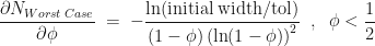
Let’s repeat the derivation but with a different cut-point e.g. 25% along the current interval bracketing the root. In general we can test whether the root is to the left of right of a point that is a proportion $\phi$ along the current interval, meaning the cut-point is $x_{lower} + \phi (x_{upper}-x_{lower})$ . At each iteration we don’t know in advance which side of the cut-point the root lies until we test for it, so in trying to determine in advance the number of iterations we need to run, we have to assume the worst case scenario and assume that the root is still in the larger of the two intervals. The reduction in uncertainty is then, ${\rm max}\{\phi, 1-\phi\}$ . Repeating the derivation we find that we have to run at least,

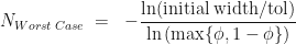
$\displaystyle N_{Worst\;Case}\;=\;\ -\frac{\ln({\rm initial\;width/tol})}{\ln\left ({\rm max}\{\phi, 1 - \phi \right \})}$

iterations to be guaranteed that we have located the root to within $tol$ .

Now to determine the cut-point $\phi$ that minimizes the upper bound on number of iterations required, we simply differentiate the expression above with respect to $\phi$ . Doing so we find,

$\displaystyle \frac{\partial N_{Worst\;Case}}{\partial \phi} \;=\; -\frac{\ln({\rm initial\;width/tol})}{ (1-\phi) \left ( \ln (1 - \phi) \right )^{2}} \;\;,\;\; \phi < \frac{1}{2}$

and

$\displaystyle \frac{\partial N_{Worst\;Case}}{\partial \phi} \;=\; \frac{\ln({\rm initial\;width/tol})}{\phi \left ( \ln (\phi) \right)^{2}} \;\;,\;\; \phi > \frac{1}{2}$

The minimum of $N_{Worst\;Case}$ is at $\phi =\frac{1}{2}$ , although $\phi=\frac{1}{2}$ is not a stationary point of the upper bound $N_{Worst\;Case}$ , as $N_{Worst\;Case}$ has a discontinuous gradient there.

That is the behaviour of the worst-case scenario. A similar analysis can be applied to the best-case scenario – we simply replace $max$ with $min$ in all the above formula. That is, in the best-case scenario the number of iterations required is given by,

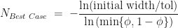
$\displaystyle N_{Best\;Case}\;=\;-\frac{\ln({\rm initial\;width/tol})}{\ln\left ({\rm min}\{\phi, 1 - \phi \right \})}$

Here, the maximum of the best-case number of iterations occurs when $\phi = \frac{1}{2}$ .

That’s the worst-case and best-case scenarios, but how many iterations do we expect to use on average? Let’s look at the expected reduction in uncertainty in the root location after $N$ iterations. In a single iteration a root that is randomly located within our interval will lie, with probability $\phi$ , in segement to the left of our cut-point and leads to a reduction in the uncertainty by a factor of $\phi$ . Similarly, we get a reduction in uncertainty of $1-\phi$ with probability $1-\phi$ if our randomly located root is to the right of the cut-point. So after $N$ iterations the expected reduction in uncertainty is,

$\displaystyle {\rm Expected\;reduction}\;=\;\left ( \phi^{2}\;+\;(1-\phi)^{2}\right )^{N}$

Using this as an approximation to determine the typical number of iterations, we get,

$\displaystyle N_{Expected\;Reduction}\;=\;-\frac{\ln({\rm initial\;width/tol})}{\ln\left ( \phi^{2} + (1-\phi)^{2} \right )}$

This still isn’t the expected number of iterations, but to see how it compares Figure 2 belows shows simulation estimates of $\mathbb{E}\left ( N \right )$ plotted against $\phi$ when the root is random and uniformly distributed within the original interval.

The number of iterations needed for the bisection algorithm — Number of iterations required for the different root finding methods.

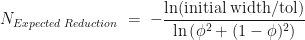
For Figure 2 we have set $w = ({\rm initial\;width/tol}) = 0.01$ . Also plotted in Figure 2 are our three theoretical estimates, $\lceil N_{Worst\;Case}\rceil, \lceil N_{Best\;Case}\rceil, \lceil N_{Expected\;Reduction}\rceil$ . The stepped structure in these 3 integer quantities is clearly apparent, as is how many more iterations are required under the worst case method when $\phi \neq \frac{1}{2}$ .

The expected number of iterations required, $\mathbb{E}( N )$ , actually shows a rich structure that isn’t clear unless you zoom in. Some aspects of that structure were unexpected, but requires some more involved mathematics to understand. I may save that for a follow-up post at a later date.

The Manchester football team that conquered the world – but you probably haven’t heard of them

On July 7, 2022August 9, 2022 By dchoyleIn Uncategorized5 Comments

Q: Which was the first Manchester football team to win a European Championship?

A: Manchester United right? Won the European Cup in 1968. No, not quite right.

This is a story about a Manchester team that swept all before them, winning a European Championship in 1957, before going on world tours, beating all the competition they encountered and playing in front of crowds of 50,000 – 60,000 spectators along the way.

The story has humble beginnings – Fog Lane Park in south Manchester. The photo above is of the duck ponds in the park, and yes, they are relevant to the story.

The founding of Manchester Corinthians

In 1949 Percy Ashley, a football scout for Bolton Wanderers, set up a women’s football team, Manchester Corinthians LFC, primarily so that his daughter Doris could play football. This was in an era when the Football Association (FA) had prohibited women from playing on pitches of FA affiliated clubs – effectively a ban on women’s football that lasted from 1921 up until 1971.

The Corinthians home ‘ground’ was Fog Lane Park. They did their training sessions there on Sundays. On poor quality muddy pitches, typical of a municipal park. Despite this, within a few years Corinthians were beating every team they encountered. By 1951 they had won the Southern Cup, the Manchester Area Cup, the Sports Magazine Cup, the Roses Trophy, the Midland Trophy, the Cresswell Trophy, the Odeon Championship Trophy, the Belle Vue Trophy, and the Festival of Great Britain Trophy.

In 1957 Corinthians were invited to represent England in a European championship, which they duly won, beating Germany 4-0 in the final. Bert Trautmann acted as Corinthian’s interpreter during the championship – yes that Bert Trautmann, the Manchester City goalkeeper who famously broke his neck partway through the 1956 FA Cup Final and carried on playing the rest of the match.

A tour of Portugal and a 3-month tour of South America followed. In Portugal Corinthians played against Benfica, with a 50,000 crowd watching. The South American tour saw crowds of 50,000 – 60,000. Former Corinthian player Margaret Whitworth recalls having to wait for the President of the country they were playing in (possibly Venezuela) to arrive by helicopter before their match could start.

The success of Corinthians was such that to find a team of similar standard against whom they could play, they had to create another Fog Lane Park based team, Nomads, formed in 1957. Nomads were just as brilliant as the Corinthians. The Corinthians and Nomads were interchangeable, rather than being a 1^st team and a reserve team. As this 1961 snippet below from the Crewe Chronicle newspaper indicates, organizers of women’s football matches would arrange for Corinthians to play Nomads, possibly because they were the two best teams in the area.

Advertisement for a Corinthians vs Nomads match. Taken from the Crewe Chronicle, May 1961.

By 1965, Corinthians had played 394 matches, winning 353 of them and losing only 20. That is a phenomenal win rate! Likewise, Nomads had played 68, won 47 and lost 11.

The success continued. 1970 saw Corinthians being invited to France to compete in a tournament against top continental European clubs, such as Italian club Juventus, Czechoslovakian champions Slavia Kaplice, and French hosts Stade de Reims. Corinthians won the tournament, beating Juventus 1-0 in a tightly contested final.

At this point Corinthians are arguably the best women’s team in England and among the best in Europe. This was at a time when women’s football in France and Italy was not banned but actively supported. The European clubs Corinthians were competing against had significant advantages in terms of quality of facilities and pitches.

In stark contrast, Corinthian players recall having to carry buckets of water from the coach’s house on Fog Lane for washing after training sessions and matches. And if the buckets of water weren’t available, they had to wash in the duck ponds (in the picture), sometimes even having to break the ice on the ponds first.

One of the Corinthian players, Jan Lyons, later went on to play for the Italian club Juventus and has remarked on the differences in facilities between women’s football in England and women’s football in Italy at the time.

The Corinthians and Nomads continued up until 1982 and were two of the 44 founding teams when the Women’s Football Association was formed in 1969/1970, meaning that just under 5% of founding teams came from a small municipal park in south Manchester.

An almost forgotten story

Surprisingly, this is a story I hadn’t heard before until a few months ago, even though I’ve lived for over 15 years on the doorstep of where it all took place – the duck ponds are 150m as the crow flies from where I’m sitting writing this in my kitchen.

It is also surprising, as my eldest daughter played football in Fog Lane Park for nearly 10 years, on those same pitches, for the local team, Didsbury Juniors, who are based out of the park. During this time my daughter was one of only two female players in what was unofficially a boys’ team. My daughter then went onto play for Manchester City Girls team and Stockport County LFC, yet in all my time connected to girls’ football in Manchester I never came across the Corinthians story.

I found out about the story when The Friends of Fog Lane Park group was contacted by football historian Gary James about putting up a plaque to commemorate the achievements of the Corinthians club. I was astounded when I heard this piece of local history – like many people in the Fog Lane/Didsbury area that I’ve spoken to since and who similarly knew nothing of the Corinthians story.

I’ve only given a small excerpt here about the Corinthians story. What I’ve written cannot really do justice to this fascinating and incredible story, so please do read more about it. For my source material I’ve used the excellent works by Gary James who has written extensively about football in the Manchester area including numerous articles about the Corinthians, and the comprehensive recent book¹ and 2019 academic paper² by Jean Williams. I’ve also used various other websites, such as here, here and here.

A permanent commemoration

The Friends of Fog Lane Park group, along with Manchester City Council and MCRactive, are raising money for a permanent reminder and celebration of the achievements of the Corinthians and Nomads teams. This is being done with the help and support of Gary James. The aim is for this commemoration to hopefully coincide with the UEFA Women’s Euros 2022, which are taking place in England during July this year. If you wish, you can donate to the fundraising at this JustGiving page. Your support would be very much appreciated.

As part of this effort to raise funds I had the pleasure of meeting with three former Corinthians (see photo below) in May this year. Naturally, the meeting took place in Fog Lane Park.

Former Corinthian players in May 2022. L-R are Jan Lyons, Margaret Shepherd (Tiny), and Margaret Whitworth (Whitty).

During the meeting the players recounted their memories of Percy and Doris Ashley, having to wash in the duck ponds, and playing for Juventus after transferring from Corinthians. One of the players also recounted that when buying football boots, they had to pretend that the boots were for hockey or lacrosse, in order for the shopkeeper to be willing to sell the boots to them, such was the social stigma against women’s football that the men’s FA had created during the period.

My thanks in writing this post go to Pam Barnes and Alice Moody for supplying material related to the Corinthians story, introducing me to the story, and many interesting conversations about it.

Footnote 1: J. Williams, The History of Women’s Football, 2019. Pen & Sword Books Ltd, Barnsley, UK. https://www.pen-and-sword.co.uk/The-History-of-Womens-Football-Hardback/p/19214.

Footnote 2: J. Williams, ‘We’re the lassies from Lancashire’: Manchester Corinthians Ladies FC and the use of overseas tours to defy the FA ban on women’s football, Sport in History 39(4):395-417, 2019. https://doi.org/10.1080/17460263.2019.1678068

Part 3 – What does the future hold?: Using forecasting in a commercial environment

On February 15, 2022December 3, 2023 By dchoyleIn Data Science, Forecasting, TimeSeriesLeave a comment

This is the last in my series of posts on forecasting. The posts have focused on the ‘why’ of forecasting and also some of the practicalities of forecasting. This last post is going to be shorter. It is simply some links to forecasting resources that I’ve found useful or think could be useful – books, articles, online tutorials and software, as well as my opinions on which bits you should focus on learning.

Books/Articles

Forecasting: Methods and Applications by Spyros Makridakis, Steven Wheelwright and Rob Hyndman. This was the book that was recommended to me by a colleague when I started in commercial forecasting. Rob Hyndman (one of the authors) says it is out of date, and recommends his later textbook (see next), but I still find it useful.
Forecasting: Principles and Practice by Rob Hyndman and George Athanasopoulos is considered one of the modern bibles on classical forecasting techniques. It is now in its 3^rd edition and also available online for free.
Introductory Time Series with R by Paul Cowpertwait and Andrew Metcalfe. I found this short but concise Springer book (in the Use R! series) on classic time-series analysis in R a great help. It was useful both from an R perspective, but also for short practical introductions and explanations of the various ARIMA concepts. Some of the links to the datasets used are now broken apparently, but I have seen comments that the resources are not hard to find with a google search.
This recent and comprehensive review article in the International Journal of Forecasting is great (arxiv version here). It has short readable paragraphs and sections on a large number of concepts and forecasting topics, so you can simply pick the topic you’re interested in and read just that. Or read the whole article end-to-end if you want.

Blogs

Rob Hyndman’s blog is the main blog I tend to routinely look at. It is always an excellent read and contains links to blogs that Hyndman recommends (although these tend to be more econometrics and statistics focused).

Software

I’m only going to give links to free open-source software. There are some other excellent commercial applications available, but not everyone will be able to get access to them, so I won’t list them.

R: I have tended to do most of my classical time-series analysis in R. The in-built arima functions and also the forecast package (created by Rob Hyndman and Yeasmin Khandakar) provide a great deal of functionality and are my go-to packages/functions in R for time-series.
The statsmodels package in python provides a similar model building experience to building models in R. Consequently, its time-series functionality provides similar capabilities to that found in R.
Darts package in python: I have done less time-series analysis in python than I have in R. When I have done exploratory time-series analysis in python I have tended to use statsmodels. Having said that, the Darts package, and the Kats package (from Facebook) look like useful python packages from the bits I have read.
Prophet package: The Prophet package, from Facebook, is open-sourced, flexible and very powerful. I have tried it for a couple of tasks. Under the hood it is based upon the Stan probabilistic programming language (PPL), which I have used a lot (both in and outside of my main employment). Prophet is fully automated but I would still recommend you have a basic grasp of classical time-series analysis concepts before you use Prophet, to guard against those situations where a fitted model is inappropriate or clearly wrong.
The engineering team at Uber have also released their own forecasting package, Orbit, which performs Bayesian forecasts using various PPLs under the hood (similar to the way the Prophet package uses Stan).

Methods/Concepts/Techniques you should know about

ARIMA: You should definitely become familiar with the classical approaches to time-series analysis, namely ARIMA. The name is a combination of acronyms, and I’ve given a breakdown of the full acronym and what I think are the important aspects to know about.
- AR: Auto-Regressive. These are the ‘lag’ terms in the time-series model equation, whereby the response variable value at timepoint t can depend on the value of the response variable at previous time-points. It is important to understand, i) how the value of the lag coefficients affect the long-run mean and variance of the response variable, including how this determines whether a process is stationary or not, ii) how to determine the order of the AR terms, e.g. by looking at a Partial Auto-Correlation Function (PACF) plot, iii) how the AR terms are infinite impulse response (IIR) terms, in contrast to the finite impulse response (FIR) moving average terms.
- I: Integrated. This is the concept within ARIMA that most Data Scientists are least familiar with but a very important one, particularly when dealing with quantities that we naturally expect to grow over time, for example by accumulating increments that increase on average. It is important to understand, i) how to run unit-root tests to test for integrated series – beware the difference between Phillips-Perron (PP) and KPSS tests, as the null hypothesis is different between them, ii) Cointegration and spurious regression (spurious correlation) – for which Clive Granger won a Nobel memorial prize in Economics (shared with Robert Engle) in 2003.
- MA: Moving Average. These are the ‘error’ terms in the time-series model equation, whereby the response variable value at timepoint t can be affected by the stochastic error not just at t, but at previous timepoints as well. This allows the response variable to be affected by short timescale perturbations of finite duration (hence the classification of the moving average terms as being finite impulse response terms).
Even if you intend to use only neural network approaches to forecasting, or want to use, say, the Prophet package as an AutoML forecasting solution, it is still a good idea to get a good grasp of ARIMA models. Investing some time in getting to grips with the basics of ARIMA and doing some hands-on playing with ARIMA models will pay huge dividends.
Error Correction Models (ECMs). You may never have need to use Error Correction Models, but they are useful for incorporating the transient departures from a long-term equilibrium. I found these University of Oxford summer school lectures notes given by Prof. Robin Best from Binghamton University (SUNY) a very good and accessible introduction to error correction models. The lecture notes also give excellent explanations of the concepts of integration and co-integration in time-series analysis. I used these lecture notes when I was having to develop an ECM for a long-range stress-testing model.
Neural Network and other Machine Learning techniques: Neural networks have been applied to time-series for a long time, but being blunt, until the last 7 years or so they weren’t very good and didn’t outperform the classical time series approaches (in my opinion). In part that was probably because machine learning practitioners tended to view time-series analysis and forecasting as ‘just another prediction problem’, and so the approaches didn’t really take into account the time-series nature of the data, e.g. the auto-regressive structure, the very things that make time-series what they are. Coupled with the fact that the classical time-series analysis approaches have a very solid theoretical underpinning in ARIMA (expressed in terms of the lag or backshift operator), this meant that machine learning approaches didn’t make as many inroads into time-series analysis as they did in other fields. However, with the advent of Deep Learning approaches using Recurrent Neural Networks and LSTM units, machine learning approaches to time-series analysis have really begun to make their mark. Models such as the DeepAR model from Salinas et al are now considered to outperform classical approaches for specific tasks. Hyndman’s book, “Forecasting: Principles and Practice” contains a chapter on machine learning approaches to time-series analysis, but in my opinion it is only very basic. The extensive review article by Petropoulos et al has a section on ‘Data-Driven Methods’ that includes sub-sections on Neural Networks and also Deep Probabilistic Forecasting Models. However, given the comprehensive nature of the whole review article these sub-sections are necessarily short. Other more extensive resources that I have found useful, which also cover the Deep Learning approaches include,
- This survey paper by Lim and Zohren.
- Lina Faik has an excellent and very up-to-date two-part blog-post on DeepAR and other seq2seq based approaches (Part 1 here, Part 2 here – on Medium) .
- There is a nice introductory TensorFlow tutorial on time-series forecasting with Neural Networks (including notebooks).
- This blog-post from Google on interpretable deep learning for time series forecasting.

That is it. I hope you have enjoyed this series of posts on forecasting. As with anything in Data Science, forecasting isn’t a spectator sport. The best way to learn is to download some datasets and start playing. You will make mistakes, but that is how you learn.

Part 2 – What does the future hold? : Using forecasting in a commercial environment

On January 11, 2022July 4, 2022 By dchoyleIn Data Science, Forecasting, TimeSeriesLeave a comment

<TL;DR>

This is part 2 of 3 about producing forecasts in real-world situations. Part 1 was more about the ‘what’ of forecasting, and specifically about different forecast horizons and how those different horizons shape how you do the forecast and what you can do with it. Part 2 is advice to help you avoid common mistakes when producing a forecast.

There are multiple distinct stages to producing and using a forecast. At the simplest level, we can list these different stages as,

Planning a forecast.
Executing a forecast.
Assessing a forecast.
Taking actions or decisions informed by a forecast.
Updating a forecast.
Deploying a forecasting process.

I have found that overwhelmingly the majority of mistakes I’ve made or seen made, are in the planning stage of producing a forecast. In fact, mistakes that I’ve seen in many of the later stages can ultimately be traced back to a failure to plan appropriately. That is, mistakes were made and spotted in one of the later stages, but if we’d thought about it properly, we could have anticipated that the error or issue would occur due to the way the forecasting process had been planned. This introduces our main takeaway,

Put a lot more time and effort into planning the forecasting process than you were initially going to do

</TL;DR>

Let’s get started. Since the majority of errors I’ve seen (and therefore opportunities for learning) are in the planning stage, that is where I’m going to focus most of my discussion. In fact, I am going to simplify the 6 stages outlined to above to just 3 broad areas of discussion,

Mistakes to avoid when planning a forecast
Mistakes to avoid when executing a forecast
Mistakes to avoid when assessing a forecast

In each of those broad areas I’ll introduce a couple of common issues or mistakes that tend to get made, and also provide some hints on how to solve the issues or avoid the mistakes – the issues and solutions will be underlined to highlight them. I’ll also drop in a couple of real-world examples where I’ve seen these mistakes made, or where I made them myself.

Planning

Model Scope:

Issue: The initial information supplied to you is never sufficient to perform an appropriate forecast. This is an unwritten first rule of forecasting¹.

There will always be important/crucial things the person requesting the forecast has not told you – out of ignorance or absent-mindedness. This is the time to ask those extra questions, such as,
1. Why do you need the forecast? What problem are you actually trying to solve? More importantly, what decision are you trying to make using the information the forecast will give?
2. How are you going to consume the forecast? Is it for insight – identifying the drivers that have the biggest impact on a medium-range outcome? Or is it for strategic planning? Or is it to be incorporated into a machine learning pipeline with an action automatically determined from the result of the forecast, e.g. changing an offer to a segment of customers.
3. What is the forecast horizon over which you need the forecast?
4. At what level of time granularity and segmentation do you need the forecast?
Solution: The answers to a) – d) above are inter-related, i.e. the answer to one may uniquely determine the answer to one of the others, but you should still ask each of those questions individually.

By understanding the scope of a system and how the forecast output is actually going to be used we avoid errors such as, failing to identify when the use-case does not justify the time and effort to develop the proposed forecasting model. A good example of this I’ve seen was a model developed for a national social housing charity that needed to predict the future costs of repairs to its housing stock. Due to various operational sensitivities, actions off the back of this prediction could only be taken at the regional level – the charity only needed to predict what the next month’s total repairs costs would be for each region in the country. But …the solution that was built used xgboost to predict the likely repair costs for each house in a region, given details about each house, and then simply aggregated the total predictions to regional level. Over the time horizons being forecasted the housing stock in each region was stable, so an equally accurate forecast could be obtained by using just the actual historical total monthly repair costs. As the historical total monthly repair costs just displayed seasonality and trend, a simple piece of SQL gave a prediction as accurate on a holdout sample as the xgboost based model.

Model Inputs:

Issue: Will you actually know all the input values and model parameter values at forecast time? Check that the values of all the exogenous variables will be known ahead of running the main forecasting model. If the exogenous variables you’ve used in your model include macro-economic quantities, their future values will not be known and you will either need a separate forecasting model for these, or their values will need to be part of the forecast scenario specification. This may be what you intended all along, but you’d be surprised how often someone builds a forecasting model and only afterwards realizes the challenges in specifying the input variables.

This problem can occur even in seemingly benign situations. For example, one mistake I’ve made in the past is using a set of dummy variables to model cohort fixed effects for a model of default rates in a loans portfolio. The only problem was that the loan book was still open – new cohorts were still coming onto the loan book – so to forecast the future default rate of the portfolio required assigning fixed effects to future, as yet unobserved, cohorts. In this instance we chose to make assignment of the future cohort effects part of the scenario specification – scenarios designated future cohorts as ‘high risk’, ‘medium risk’ or ‘low risk’ with the effects values being calculated from an appropriate centile of the historic cohort effects estimates. An alternative approach might have been to treat the cohort effects as random effects and when forecasting marginalize over the random effects of future cohorts. However, the two takeaways from this are, i) when planning a forecast model, think ahead to when you’re going to use it to produce the forecast and make sure you know how you’re going to obtain the input variables, ii) be cautious about including fixed cohort effects when producing forecasts for a changing cohort mix.

Solution: Mentally run through the forecasting process in your head, or on paper, before you start estimating your models. This will flush out issues with the model form or forecasting technique before you have committed to building them.
Issue: Variables/features not included in the model in a sensible or correct form.

I’ve a seen a model built by a marketing team that predicted the response to marketing activity. It was suspected that weather had an impact on how effective the marketing was. This was not an unreasonable hypothesis – when the summer weather is hot and sunny (not that common in the UK) most people want to be outside, in the park or at the beach, not paying close attention to some TV advert. The only problem was that ‘weather’ had been included in the predictive model as the average monthly temperature across the whole of England. There are so many things wrong with this,

The temperature in England on a single day can vary hugely from one place to another. It can be sunny and 25°C in London whilst it is raining and 15°C in Manchester and hailing and 10°C in Newcastle. The England-wide average is a meaningless feature to try and reflect how likely anybody in a specific geography is to respond to marketing. The people in London will be relaxing in the park, ignoring the TV adverts, whilst people in Newcastle will be putting an extra jumper on and hunkering down in front of soap re-runs on the TV.
In a similar vein, the use of a monthly average temperature is pointless. It was believed that the impact of weather on the marketing effectiveness was because of un-seasonal sunny weather over a few days. A monthly average will not reflect this. The monthly England-wide average temperature will reflect just seasonal patterns, not the particular effect the stakeholder was trying to understand.
Temperature is the wrong feature to use here. Hours of sunlight may be better, since the hypothesis was that it was the un-expected very sunny summer weather that was reducing the effectiveness of the marketing. Even better, a feature that captured the presence of unusually hot, dry weather on summer days would be preferable to include in the model. Note that we have now moved from discussing temperature to talking about ‘dry’ summer days, i.e., the absence of any precipitation. When including weather effects in a model it can even be crucial to think what form of precipitation is relevant here. A former colleague told me about some work he’d done for a British mobile phone operator. The mobile company was interested in the impact of weather as they’d noticed that call volumes increased sometimes when there was precipitation. The analysis revealed that, yes, precipitation had an impact, but the form of the precipitation is hugely important. If it’s raining the impact is small, but lower the temperature so that the precipitation comes in the form of snow and the call volumes spike – everybody is phoning home or phoning work to say they are delayed because of snow-blocked roads or trains not running because of ice and snow on the rails. The lesson here is that the precise way in which weather affects our outcome of interest needs to be understood.
Lastly, weather is a prime example of a variable that we won’t automatically know when it comes to producing the forecast. We may have a brilliant forecasting model, but we need to forecast the specific weather feature as well and we may not be able to do that accurately enough to get the benefit of our main forecasting model.

It was suspected that the person who built the model I’ve described just threw ‘weather’ into the model because they were told to. They simply got hold of the easiest or most accessible single weather variable they could find.

Solution: Spend time thinking through the form or particular variant of the feature you are putting into your forecasting model. Will it actually be capable of reflecting the actual effect you are trying to capture in your model? Is it at the right temporal and spatial granularity to be able to do that?

Issue: Insufficient length of training data. Make sure the length of historical data you use to build your forecasting model is sufficiently long. How long is ‘sufficiently long’? Paul Saffo in this 2007 Harvard Business Review article on the 6 Rules For Effective Forecasting says that you should “look back twice as far as you look forward”. I would say you should look back even further. The point here, however, is not to give a precise rule for how much historical data you need for a given forecast horizon, but more to emphasize that the length of historical data you should use is always longer than you think. It should be sufficiently long enough to display several examples of the phenomena you need to capture with your model. To give an example – if you are modelling the effects of macro-economic climate on a financial metric, e.g., loan default rates, then you will want to include several business cycles and more importantly several recessionary periods in your historical training data. How far back in history is still a matter of subjective judgement – for example, was the recession resulting from the 2008 financial crash typical or atypical of the dynamics you want to model and forecast? This highlights two points, i) how far you go back in history can require a detailed discussion and review of the historical data – it is not simply, ‘let’s just include the last two recessions’, ii) you need to have a good idea of what sort of phenomena and/or dynamics you need to model for your forecasts to be representative of the scenarios you are trying to understand. Use the wrong data and the usefulness of your forecasting model may be short-lived. For long-range forecasts you’ll never really know in advance the full range of phenomena that your model needs to capture, as unpredictable and impactful phenomena are always capable of arising within the forecast horizon of a long-range forecast – what are called ‘Black-Swan’ events in parts of the popular science literature. In Part 1 we explained that by considering a very wide range of scenarios we mitigate against this, to a degree. But it means that a model used for long-range forecasting has to have captured dynamics and behaviour appropriate to a very wide range of phenomena – and that can require an awful lot of historical data. Anecdotally, I’ve seen that the length of training data required increases super-linearly with the length of the forecast horizon.

Solution: Think about the kind of phenomena or scenarios you want your model to be capable of forecasting. Does your training data contain adequate examples of such phenomena or scenarios? If yes, then you probably have enough training data. If no, then get additional appropriate training data, or shorten your forecast horizon (see Part I for why you should do this).

Model Form:

Issue: Using a complex or unusual generative modelling technique and believing you can just include the predictive features into the ‘model’ as you would when building a linear model or GLM.

I have seen an agent-based model used to attempt to forecast and identify emergent phenomena that it was believed would occur in response to a macro-economic change or shock. The agent-based simulation was used to mimic the microscopic interactions between the agents and their external environment – the general economy. A macro-economic variable, I think it was unemployment rate, was directly coupled to each agent’s propensity to spend. Lo-and-behold, when the unemployment rate increased the forecast showed that the total expenditure in the system went down. This was hailed as a new finding, showing emergent behaviour. No! It just reflected how the macro-economic variables had been included in the modelling. At this point over 12 months (at 3 FTE, I believe) had been expended on this project.

How the exogenous influences are coupled to a forecasting technique is critically important if we want to identify genuine emergent phenomena. Genuinely emergent phenomena are typically a global property of the system, often resulting from a global constraint. For example, in a physical system it could be a requirement to minimize the overall free energy of the system. In a financial system it could be a requirement to maximize total profit. Ideally, we should think about how the exogenous influences interact with these global constraints when including the exogenous variables in our modelling. If instead the exogenous variables are coupled directly to a metric we will later measure, we should not be surprised when that metric changes when the exogenous variables do.

Solution: The more complex the technique used you more you’ll need to think about how you put the predictive features into the ‘model’.
Issue: Computational optimization of forecast model outputs will exploit the weaknesses in your model. Be aware of the potential future downstream uses of your forecasting process. The forecasting technique you’ve used may not be robust enough to support likely (and anticipatable) downstream uses. It is likely, you’ve set up your forecasting process as an automatable, reproducible codebase. That codebase can then be included in a downstream automated process, such as finding the optimal value of one the actionable input variables. The optimization process will optimize the output of the forecasting model and because forecasts are, almost by definition, ‘out-of-sample’, there is the potential for the optimization process to drive the model to a region of the input space where the model output is non-sensical. This is because the optimization process does not know any better – we have not ensured that the forecasting model output has sensible and credible behaviour for all scenarios or for all sets of input values. To do this we need to build sensible structural constraints or principles into our forecasting model. Such constraints or principles usually come from domain knowledge, e.g. from economic principles when building forecasting models that include macro-economic inputs. These constraints or principles represent assumptions – we are assuming that our system of interest will or should obey classical economic principles. If those assumptions are incorrect, we will be guilty of produced a biased forecast. How do we know when to include such constraints or principles? We don’t know precisely, but we can think before constructing the forecasting model whether the benefits of including them outweigh the dis-advantages, and we are forewarned as to the potential bias. The main point here is, again, think and plan.

Solution: Understand if you will always be in control of the uses of your model. If not, then think whether your model needs to be robust to use-cases you can’t control.

Model Estimation:

Issue: The model estimation process is not set up to reflect what you’re actually trying to model. Use a cost-function that reflects the outcome you care about. When fitting a forecasting model, we will typically be minimizing some cost-function. Choose the cost-function appropriately. If forecast accuracy is going to be assessed using a different cost-function you may want to rethink the cost-function you use for fitting. Or in simple terms, fit your model to optimize the outcome you actually care about.

Solution: Think through each step of the proposed estimation process. Is it ideal for the thing you’re trying to capture.

Execution

Issue: How do you gauge whether your forecast is credible? Always run a baseline calculation or baseline scenario. For a short-range forecast you may have characterized very precisely the scenario you wish to predict, but your baseline scenario can still be something like a Business-As-Usual (BAU) scenario. For long-range forecasting, you can also use a BAU scenario as your baseline scenario but the definition of BAU may be more subjective and contain significant movement in exogenous influences – although it probably won’t be what you consider to be the most extreme scenario. The main benefit of running a baseline scenario is that it allows you to compute realistic ‘deltas’ even if there are far-from-perfect assumptions in your forecasting methodology. Remember the quote from George Box – ‘All models are wrong, but some are useful.’ The skill as a Data Scientist/Statistician is in knowing how to extract the useful insight and information from a ‘wrong’ model. With a baseline calculation you can compute how much worse or better the outcome is under scenario X compared to the baseline scenario. As a human you may then have a feel for what is incorrect in the baseline calculation and correct it or down-weight it. The model based estimate of the delta between scenario X and baseline scenario can then be applied to the human corrected baseline.

Solution: Running a baseline scenario where you have a more intuitive feel for how the system responds will help you assess any other scenario.
Issue: We have a forecast but not a quantitative measure of how confident we are with it. Always produce measures of uncertainty, e.g. confidence intervals for your forecasts. There is limited value in just a point estimate. How sensitive is that estimate to the stochastic component of the response variable dynamics? Then on top that we have uncertainty in the forecast due to parameter uncertainty and potentially also input uncertainty. Sensitivity analysis can help us quantify the impact on the forecast from both parameter uncertainty and input uncertainty, so that we can identify which we need to improve most. Don’t assume that just because values of exogenous variables have been specified for the forecast scenario that they are accurate. Forecast scenarios that are, upfront, specified very precisely can still be mis-specified or specified inappropriately, or even subject to change – it is not unusual for a company to execute a different BAU scenario to what they said they would at the time the forecast was produced.

Solution: Quantify the impact on a forecast from all the major sources of uncertainty. Doing so is essential for framing and qualifying any decisions or actions taken on the back of the forecast output.

Issue: Distinguishing outputs from different forecasts gets messy when you have lots of them. Create a system for time-stamping forecast outputs, the associated input data and meta-data and also the codebase used to produce the forecast. This creates a disciplined process for running, re-running, and changing forecasts whilst knowing which run produced which forecast. You’ll be surprised how often you’ll end up asking yourself questions similar to , ‘now, did I include 5 or 6 years of training data and was it a 2month gap between the end of the training data and the beginning of the forecast horizon?’ Set-up a system to accurately capture what each forecast used, did, and what it was about.

Solution: Set up a system from the outset for timestamping and logging your forecast outputs along with the details on the inputs.

Assessment

Issue: How do you assess the accuracy of your forecasting method if the inputs may also be uncertain? If your forecasting model includes an input feature that itself is forecasted, then always perform holdout tests on your model with and without perfect hindsight.
1. Testing with perfect hindsight is when we perform the holdout test using the actual observed values of all the input features.
2. Testing without perfect hindsight is when we perform the holdout test using the forecasted values of any input features that need to be forecasted when actually running in production.
The clear value of performing the two different versions of the holdout tests is that it helps identify where the biggest bottleneck in forecast accuracy is. There is no point in trying to further improve a main forecasting model that is already accurate, say over a 1 year time horizon, if it is only accurate if we know all the inputs precisely and our forecasts of one of the input features is woeful – put the effort into improving the feature forecasting model.

Solution: Assess holdout forecast accuracy with and without perfect hindsight on the input variables.
Issue: How do know whether your complex forecasting technique is adding any value? Always run a baseline technique when assessing holdout accuracy. This is true of any use of machine learning. When building predictive classification models we often build a simple classifier, such as a naïve Bayes classifier, to provide a baseline against which to judge our more complex and sophisticated models and to check that the extra complexity is warranted. Similarly, when producing a forecast for a scenario using our chosen forecasting technique, we should include the forecast from a much simpler technique, such as exponential smoothing. In fact, this commentary, in the International Journal of Forecasting, on the recent M5 forecasting competition suggests 92.5% of the time you won’t beat a simple exponential smoothing model.

Solution: Include a simple baseline forecasting technique.
Issue: Over confidence in the forecast output.

Another of my favourite quotes from the famous statistician George Box,

‘Statisticians, like artists, have the bad habit of falling in love with their models.
George Box

I have been guilty of this myself. We become blind to the possibility that the output from a model can still be garbage even when we have provided high-quality input data. We believe that because we have circumvented the ‘garbage-in, garbage-out’ issue we must have a credible forecast because of the elegance and sophistication of the forecasting technique we have used. We have become seduced by the elegance of the forecasting technique. We have forgotten that ‘all models are wrong’. Well, if a model can be wrong, it can be completely and utterly wrong, and we should remember that. The first rule of forecast assessment – always doubt your forecast. Look at the forecast and see if you can explain to yourself why the forecast has that shape given the inputs.

Solution: Always be prepared to doubt and, if necessary, overrule your forecasts.

That’s Part 2. I hope it has been helpful. In Part 3 I’ll list some forecasting learning resources and tools that I’ve found useful.

Footnote 1: I seem to recall seeing this rule written in a blogpost or paper somewhere, but I’m unable to locate it. If anybody is aware of an original source for it, please let me know.

Benford’s Law

What is Benford’s Law?

What’s behind Benford’s Law

Deriving Benford’s Law

Ted Hill’s proof of Benford’s Law

Benford’s Law is base invariant

When should a dataset follow Benford’s Law?

Why computer file sizes follow Benford’s Law

The history of Benford’s Law

Simon Newcomb

Benford’s discovery

Applications of Benford’s Law

My involvement with Benford’s Law

My Python code solution

Share this:

There are two parts to this puzzle

The overall goal

The twist

Share this:

Speeding up your code with your current tech stack

Amdahl’s law

How small is S?

A real-world example

What to do?

Share this:

The Books

What the books are about

Share this:

Share this:

Statistics is about the whole data life cycle

A Strong Data Science focus

A growing Data Science presence

Other relevant sessions

The Future of the Data Science Profession

Diversity of topics across the whole conference

A friendly conference

Next year – Harrogate 2023

Share this:

<TL;DR>

</TL;DR>

Is bisection optimal?

Dividing the interval unequally

Share this:

The founding of Manchester Corinthians

An almost forgotten story

A permanent commemoration

Share this:

Books/Articles

Blogs

Software

Methods/Concepts/Techniques you should know about

Share this:

<TL;DR>

</TL;DR>

Planning

Model Scope:

Model Inputs:

Model Form:

Model Estimation:

Execution

Assessment

Share this: