An equation showing the mathematical form of the log sum exp calculation.

Data Science Notes: 2. Log-Sum-Exp

Summary

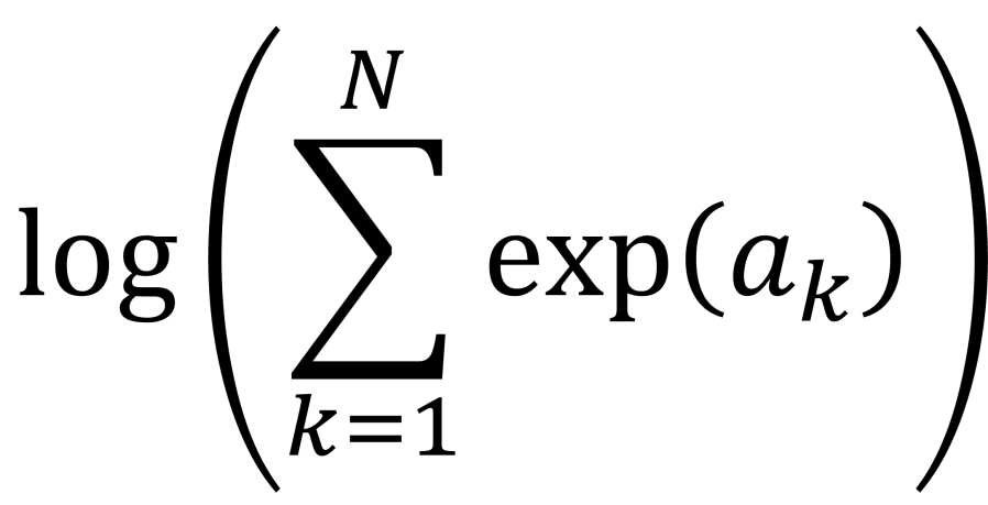
  • Summing up many probabilities that are on very different scales often involves calculation of quantities of the form \log\left ( \sum_{k} \exp\left( a_{k}\right )\right ). This calculation is called log-sum-exp.
  • Calcuating log-sum-exp the naive way can lead to numerical instabilities. The solution to this numerical problem is the “log-sum-exp” trick.
  • The scipy.special.logsumexp function provides a very useful implementation of the log-sum-exp trick.
  • The log-sum-exp function also has uses in machine learning, as it is a smooth, differentiable approximation to the {\rm max} function.

Introduction

This is the second in my series of Data Science Notes series. The first on Bland-Altman plots can be found here. This post is on a very simple numerical trick that ensures accuracy when adding lots of probability contributions together. The trick is so simple that implementations of it exist in standard Python packages, so you only need to call the appropriate function. However, you still need to understand why you can’t just naively code-up the calculation yourself, and why you need to use the numerical trick. As with the Bland-Altman plots, this is something I’ve had to explain to another Data Scientist in the last year.

The log-sum-exp trick

Sometimes you’ll need to calculate a sum of the form, \sum_{k} \exp\left ( a_{k}\right ), where you have values for the a_{k}. Really? Will you? Yes, it will probably be calculating a log-likelihood, or a contribution to a log-likelihood, so the actual calculation you want to do is of the form,

\log\left ( \sum_{k} \exp \left ( a_{k}\right )\right )

These sorts of calculations arise where you have log-likelihood or log-probability values a_{k} for individual parts of an overall likelihood calculation. If you come from a physics calculation you’ll also recognise the expression above as the calculation of a log-partition function.

So what we need to do is exponentiate the a_{k} values, sum them, and then take the log at the end. Hence the expression “log-sum-exp”. But why a blogpost on “log-sum-exp”? Surely, it’s an easy calculation. It’s just np.log(np.sum(np.exp(a))) , right ? Not quite.

It depends on the relative values of the a_{k}. Do the naïve calculation np.log(np.sum(np.exp(a))) and it can be horribly inaccurate. Why? Because of overflow and underflow errors.

If we have two values a_{1} and a_{2} and a_{1} is much bigger than a_{2}, when we add \exp(a_{1}) to \exp(a_{2}) we are using floating point arithmetic to try and add a very large number to a much smaller number. Most likely we will get an overflow error. If would be much better if we’d started with \exp(a_{1}) and try to add \exp(a_{2}) to it. In fact, we could pre-compute a_{2} - a_{1}, which would be very negative and from this we could easily infer that adding \exp(a_{2}) to \exp(a_{1}) would make very little difference. In fact, we could just approximate \exp(a_{1}) + \exp(a_{2}) by \exp(a_{1}).

But how negative does a_{2} - a_{1} have to be before we ignore the addition of \exp(a_{2})? We can set some pre-specified threshold, chosen to avoid overflow or underflow errors. From this, we can see how to construct a little Python function that takes an array of values a_{1}, a_{2},\ldots, a_{N} and computes an accurate approximation to  \sum_{k=1}^{N}\exp(a_{k}) without encountering underflow or overflow errors.

In fact we can go further and approximate the whole sum by first of all identifying the maximum value in an array a = [a_{1}, a_{2}, \ldots, a_{N}]. Let’s say, without loss of generality, the maximum value is a_{1}. We could ensure this by first sorting the array, but it isn’t necessary actually do this to get the log-sum-exp trick to work. We can then subtract a_{1} from all the other values of the array, and we get the result, 

\log \left ( \sum_{k=1}^{N} \exp \left ( a_{k} \right )\right )\;=\; a_{1} + \log \left ( 1\;+\;\sum_{k=2}^{N} \exp \left ( a_{k} - a_{1} \right )\right )

The values a_{k} - a_{1} are all negative for k \ge 2, so we can easily approximate the logarithm on the right-hand side of the equation by a suitable expansion of \log (1 + x). This is the “log-sum-exp” trick.

The great news is that this “log-sum-exp” calculation is so common in different scientific fields that there are already Python functions written to do this for us. There is a very convenient “log-sum-exp” function in the SciPy package, which I’ll demonstrate in a moment.

The log-sum-exp function

The sharp-eyed amongst you may have noticed that the last formula above gives us a way of providing upper and lower bounds for the {\rm max} function. We can simply re-arrange the last equation to get,

{\rm max} \left ( a_{1}, a_{2},\ldots, a_{N} \right ) \;\le\; \log \left ( \sum_{k=1}^{N}\exp \left ( a_{k}\right )\right )

The logarithm calculation on the right-hand side of the inequality above is what we call the log-sum-exp function (lse for short). So we have, 

{\rm max} \left ( a_{1}, a_{2},\ldots, a_{N} \right ) \;\le\; {\rm lse}\left ( a_{1}, a_{2}, \ldots, a_{N}\right )

This gives us an upper bound for the ${\rm max}$ function. Since a_{k} \le {\rm max}\left ( a_{1}, a_{2},\ldots,a_{N}\right ), it is also relatively easy to show that,

{\rm lse} \left ( a_{1}, a_{2}, \ldots, a_{N}\right )\;\le\; {\rm max}\left ( a_{1}, a_{2},\ldots, a_{N} \right )\;+\;\log N

and so we have have a lower bound for the {\rm max} function. So the log-sum-exp function allows us to compute lower and upper bounds for the maximum of an array of real values, and it can provide an approximation of the maximum function. The advantage is that the log-sum-exp function is smooth and differentiable. In contrast, the maximum function itself is not smooth nor differentiable everywhere, and so is less convenient to work with mathematically. For this reason the log-sum-exp is often called the “real-soft-max” function because it is a “soft” version of the maximum function. It is often used in machine learning settings to replace a maximum calculation.

Calculating log-sum-exp in Python

So how do we calculate the log-sum-exp function in Python. As I said, we can use the SciPy implementation which is in scipy.special. All we need to do is pass an array-like set of values a_{k}. I’ve given a simple example below, 

# import the packages and functions we need
import numpy as np
from scipy.special import logsumexp

# create the array of a_k values 
a = np.array([70.0, 68.9, 20.3, 72.9, 40.0])

# Calculate log-sum-exp using the scipy function 
lse = logsumexp(a)

# look at the result
print(lse)

This will give the result 72.9707742189605

The example above and several more can be found in the Jupyter notebook DataScienceNotes2_LogSumExp.ipynb in the GitHub repository https://github.com/dchoyle/datascience_notes

The great thing about the SciPy implementation of log-sum-exp is that it allows us to include signed scale factors, i.e. we can compute,

\log \left ( \sum_{k=1}^{N} b_{k}\exp\left ( a_{k}\right ) \right )

where the values b_{k} are allowed to be negative. This means, that when we are using the SciPy log-sum-exp function to perform the log-sum-exp trick, we can actually use it to calculate numerically stable estimates of sums of the form,

\log \left ( \exp\left ( a_{1}\right ) \;-\; \exp\left ( a_{2}\right ) \;-\;\exp\left ( a_{3}\right )\;+\;\exp\left ( a_{4}\right )\;+\ldots\; + \exp\left ( a_{N}\right )\right ).

Here’a small code snippet illustrating the use of the scipy.special.logsumexp with signed contributions,

# Create the array of the a_k values
a = np.array([10.0, 9.99999, 1.2])
b = np.array([1.0, -1.0, 1.0])

# Use the scipy.special log-sum-exp function
lse = logsumexp(a=a, b=b)

# Look at the result
print(lse)

This will give the result 1.2642342014146895.

If you look at the output of the example above you’ll see that the final result is much closer to the value of the last array element a_{3} = 1.2. This is because the first two contributions, \exp(a_{1}) and \exp(a_{2}) almost cancel each other out because the contribution \exp(a_{2}) is pre-fixed by a factor of -1. What we get left with is something close to \log(\exp(a_{3}))\;=\; a_{3}.

There is also a small subtlety in using the SciPy logsumexp function with signed contributions. If the substraction of some terms had led to an overall negative result, scipy.special.logsumexp will rerturn NaN as the result. In order to get it to always return a result for us, we have to tell it to return the sign of the final summation as well, by setting the return_sign argument of the function to True. Again, you can find the code example above and others in the notebook DataScienceNotes2_LogSumExp.ipynb in the GitHub repository https://github.com/dchoyle/datascience_notes.

When you are having to combine lots of different probabilities, that are on very different scales, and you need to subtract some of them and add others, the SciPy log-sum-exp function is very very useful.

© 2026 David Hoyle. All Rights Reserved

Faa di Bruno and derivatives of an iterated function

I have recently needed to do some work evaluating high-order derivatives of composite functions. Namely, given a function f(t), evaluate the n^{th} derivative of the composite function  \underbrace{\left (f\circ f\circ f \circ \ldots\circ f \right )}_{l\text{ terms}}(t)
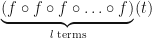
. That is, we define f_{l}(t) to be the function obtained by iterating the base function f(t)=f_{1}(t) l-1 times. One approach is to make recursive use of the Faa di Bruno formula,

\displaystyle \frac{d^{n}}{dx^{n}}f(g(x))\;=\;\sum_{k=1}^{n}f^{(k)}(g(x))B_{n,k}\left (g'(x), g''(x), \ldots, g^{(n-k+1)}(x) \right )      Eq.(1)

The fact that the exponential partial Bell polynomials B_{n,k}\left (x_{1}, x_{2},\ldots, x_{n-k+1} \right ) are available within the {\tt sympy} symbolic algebra Python package, makes this initially an attractive route to evaluating the required derivatives. In particular, I am interested in evaluating the derivatives at t=0 and I am focusing on odd functions of t, for which t=0 is then obviously a fixed-point. This means I only have to supply numerical values for the derivatives of my base function f(t) evaluated at t=0, rather than supplying a function that evaluates derivatives of f(t) at any point t.

Given the Taylor expansion of f(t) about t=0 we can easily write code to implement the Faa di Bruno formula using sympy. A simple bit of pseudo-code to represent an implementation might look like,

  1. Generate symbols.
  2. Generate and store partial Bell polynomials up to known required order using the symbols from step 1.
  3. Initialize coefficients of Taylor expansion of the base function.
  4. Substitute numerical values of derivatives from previous iteration into symbolic representation of polynomial.
  5. Sum required terms to get numerical values of all derivatives of current iteration.
  6. Repeat steps 4 & 5.

I show python code snippets below implementing the idea. First we generate and cache the Bell polynomials,

 # generate and cache Bell polynomials
 bellPolynomials = {}
 for n in range(1, nMax+1):
      for k in range(1, n+1):
         bp_tmp = sympy.bell(n, k, symbols_tmp)
         bellPolynomials[str(n) + '_' + str(k)] = bp_tmp

Then we iterate over the levels of function composition, substituting the numerical values of the derivatives of the base function into the Bell polynomials,

for iteration in range(nIterations):
    if( verbose ):
        print( "Evaluating derivatives for function iteration " + str(iteration+1) )

    for n in range(1, nMax+1):
        sum_tmp = 0.0
        for k in range(1, n+1):
            # retrieve kth derivative of base function at previous iteration
            f_k_tmp = derivatives_atFixedPoint_tmp[0, k-1]

            #evaluate arguments of Bell polynomials
            bellPolynomials_key = str( n ) + '_' + str( k )
            bp_tmp = bellPolynomials[bellPolynomials_key]
            replacements = [( symbols_tmp[i],
            derivatives_atFixedPoint_tmp[iteration, i] ) for i in range(n-k+1) ]
            sum_tmp = sum_tmp + ( f_k_tmp * bp_tmp.subs(replacements) )

        derivatives_atFixedPoint_tmp[iteration+1, n-1] = sum_tmp

Okay – this isn’t really making use true recursion, merely looping, but the principle is the same. The problem one encounters is that the manipulation of the symbolic representation of the polynomials is slow, and run-times slow significantly for n > 15.

However, the n^{th} derivative can alternatively be expressed as a sum over partitions of n as,

\displaystyle \frac{d^{n}}{dx^{n}}f(g(x))\;=\;\sum \frac{n!}{m_{1}!m_{2}!\ldots m_{n}!} f^{(m_{1}+m_{2}+\ldots+m_{n})}\left ( g(x)\right )\prod_{j=1}^{n}\left ( \frac{g^{(j)}(x)}{j!}\right )^{m_{j}}   Eq.(2)

where the sum is taken over all non-negative integers tuples m_{1}, m_{2},\ldots, m_{n} that satisfy 1\cdot m_{1}+ 2\cdot m_{2}+\ldots+ n\cdot m_{n}\;=\; n. That is, the sum is taken over all partitions of  n. Fairly obviously the Faa di Bruno formula is just a re-arrangement of the above equation, made by collecting terms involving f^{(k)}(g(x)) together, and as such that rearrangement gives the fundamental definition of the partial Bell polynomial.

I’d shied away from the more fundamental form of Eq.(2) in favour of Eq.(1) as I believed the fact that a number of terms had already been collected together in the form of the Bell polynomial would make any implementation that used them quicker. However, the advantage of the form in Eq.(2) is that the summation can be entirely numeric, provided an efficient generator of partitions of n is available to us. Fortunately, sympy also contains a method for iterating over partitions. Below are code snippets that implement the evaluation of f_{l}^{(n)}(0) using Eq.(2). First we generate and store the partitions,

# store partitions
pStore = {}
for k in range( n ):
    # get partition iterator
    pIterator = partitions(k+1)
    pStore[k] = [p.copy() for p in pIterator]

After initializing arrays to hold the derivatives of the current function iteration we then loop over each iteration, retrieving each partition and evaluating the product in the summand of Eq.(2). Obviously, it is relatively easy working on the log scale, as shown in the code snippet below,

# loop over function iterations
for iteration in range( nIterations ):

    if( verbose==True ):
        print( "Evaluating derivatives for function iteration " + str(iteration+1)  )

    for k in range( n ):
        faaSumLog = float( '-Inf' )
        faaSumSign = 1

        # get partitions
        partitionsK = pStore[k]
        for pidx in range( len(partitionsK) ):
            p = partitionsK[pidx]
            sumTmp = 0.0
            sumMultiplicty = 0
            parityTmp = 1
            for i in p.keys():
                value = float(i)
                multiplicity = float( p[i] )
                sumMultiplicty += p[i]
                sumTmp += multiplicity * currentDerivativesLog[i-1]
                sumTmp -= gammaln( multiplicity + 1.0 )
                sumTmp -= multiplicity * gammaln( value + 1.0 )
                parityTmp *= np.power( currentDerivativesSign[i-1], multiplicity )	

            sumTmp += baseDerivativesLog[sumMultiplicty-1]
            parityTmp *= baseDerivativesSign[sumMultiplicty-1]

            # now update faaSum on log scale
            if( sumTmp > float( '-Inf' ) ):
                if( faaSumLog > float( '-Inf' ) ):
                    diffLog = sumTmp - faaSumLog
                    if( np.abs(diffLog) = 0.0 ):
                            faaSumLog = sumTmp
                            faaSumLog += np.log( 1.0 + (float(parityTmp*faaSumSign) * np.exp( -diffLog )) )
                            faaSumSign = parityTmp
                        else:
                            faaSumLog += np.log( 1.0 + (float(parityTmp*faaSumSign) * np.exp( diffLog )) )
                    else:
                        if( diffLog > thresholdForExp ):
                            faaSumLog = sumTmp
                            faaSumSign = parityTmp
                else:
                    faaSumLog = sumTmp
                    faaSumSign = parityTmp

        nextDerivativesLog[k] = faaSumLog + gammaln( float(k+2) )
        nextDerivativesSign[k] = faaSumSign

Now let’s run both implementations, evaluating up to the 15th derivative for 4 function iterations. Here my base function is f(t) =1 -\frac{2}{\pi}\arccos t. A plot of the base function is shown below in Figure 1.
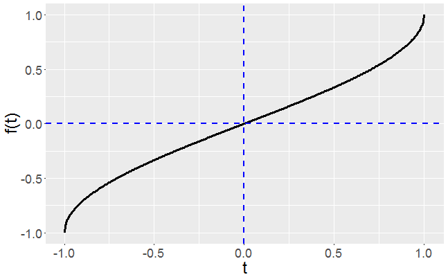
FaaDiBrunoExample_BaseFunction
Figure 1: Plot of the base function f(t)\;=\;1\;-\;\frac{2}{\pi}\arccos(t)

The base function has a relatively straight forward Taylor expansion about t=0,

\displaystyle f(t)\;=\;\frac{2}{\pi}\sum_{k=0}^{\infty}\frac{\binom{2k}{k}t^{2k+1}}{4^{k}\left ( 2k+1 \right )}\;\;\;,\;\;\;|t| \leq 1 \;\;,    Eq.(3)

and so supplying the derivatives, f^{(k)}(0), of the base function is easy. The screenshot below shows a comparison of f_{l}^{(15)}(0) for l\in \{2, 3, 4, 5\}. As you can see we obtain identical output whether we use sympy’s Bell polynomials or sympy’s partition iterator.

FaaDiBruno_TimingComparison

The comparison of the implementations is not really a fair one. One implementation is generating a lot of symbolic representations that aren’t really needed, whilst the other is keeping to entirely numeric operations. However, it did highlight several points to me,

  • Directly working with partitions, even up to moderate values of n, e.g. n=50, can be tractable using the sympy package in python.
  • Sometimes the implementation of the more concisely expressed representation (in this case in terms of Bell polynomials) can lead to an implementation with significantly longer run-times, even if the more concise representation can be implemented concisely (less lines of code).
  • The history of the Faa di Bruno formula, and the various associated polynomials and equivalent formalisms (such as the Jabotinksy matrix formalism) is a fascinating one.

I’ve put the code for both methods of evaluating the derivatives of an iterated function as a gist on github.

At the moment the functions take an array of Taylor expansion coefficients, i.e. they assume the point at which derivatives are requested is a fixed point of the base function. At some point I will add methods that take a user-supplied function for evaluating the k^{th} derivative, f^{(k)}(t), of the base function at any point t and will return the derivatives, f_{l}^{(k)}(t) of the iterated function.

I haven’t yet explored whether, for reasonable values of n (say n \leq 50), I need to work on the log scale, or whether direct evaluation of the summand will be sufficiently accurate and not result in overflow error.