In another post I had to find the eigenvalues and eigenvectors of the following matrix,

where 


In that original post I said that diagonalizing this matrix (finding its eigenvalues and eigenvectors) was easy. A colleague asked me why I thought it was easy. My answer, “well because it is the only matrix form whose eigen-decomposition I explicitly remember”. And there’s a reason why I remember how to decompose by hand these types of matrices,
- It is easy to do.
- These types of matrices are very common.
Okay, I know that reason 1 is a circular argument, but it’s true. These types of matrices are easy to diagonalize and you’ll agree when you learn the trick to calculate their eigenvalues and eigenvectors. And like all the posts in my Data Science Notes series, I’m basing this post on experience. It is nearly 29 years since I first learnt this trick, and I have used it many time since. The reason I find it so useful is because of reason 2 above.
Reason 2 is equally important. As a Data Scientist you will encounter this form of matrix often, and so there is an advantage to knowing how to calculate the eigenvectors and eigenvalues of a matrix such as 
Let’s begin. To start we’ll need to do a quick recap of what an eigenvector is and what an eigenvalue is.
Recap of what eigenvectors and eigenvalues are
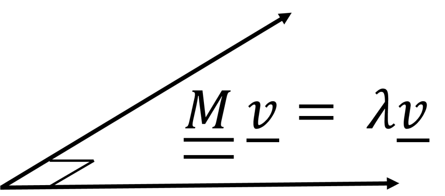
An eigenvector 

The scalar quantity 


An 


The eigen-decomposition of a matrix
We can see from Eq.2 that the effect of the matrix

And once we have all the eigenvectors 


Identifying our eigenvectors
Now, our goal is the work out the eigenvalues and eigenvectors of the matrix,

In Eq.6 I have generalized from the matrix form in Eq.1 a little here, so we have 

Let’s write the right-hand-side of Eq. 6 as a sum of two matrices, i.e. we write,

with the matrix 

This leads us to our first trick. If we have a vector 

Eq.9 tells us that eigenvectors of
Now we introduce our second trick. We look at the definition of 

Ok, but we only have 


So any vector orthogonal to all the vectors
Now we can combine our first and second tricks together the finally work out the eigenvectors and eigenvalues of
Eigenvalue = 

Eigenvalue = 

……
Eigenvalue = 

Eigenvalue = 
Putting it all together
Let’s put this into action. Let’s go back to our original matrix in Eq.1 at the start of this post. That matrix was of the form,
So comparing Eq.11 to Eq.6 we have 


Eigenvalue 1 = 

Eigenvalues 2 to
We can now easily calculate the determinant of our matrix in Eq.1 and we get,

We can also easily calculate the inverse of the matrix in Eq.1. In this case we get,

In Eq.13 the vectors 
Now, we can use one final little trick to simplify the right-hand-side of Eq.13. If we recall that the effect of the identity matrix 


Now Eq.14 is almost what we have in the first term on the right-hand-side of Eq.13. Our sum in Eq.13 runs from 


where the vectors 


Combining this with the final term on the right-hand-side of Eq.13 we get our final simplified expression for 

That’s it. If you want a challenge to test your understanding, then using the ideas and tricks we introduced above see if you can construct a closed form expression for the inverse of the matrix in Eq.6, not just the special case of the matrix in Eq.1.
Other low-rank perturbation tricks
In my original post I wanted to find the eigenvectors and eigenvalues of the matrix in Eq.1. I’ve also illustrated that once we have closed-form expressions for the eigenvectors and eigenvalues we can calculate the determinant and inverse of
- Sylvester’s determinant theorem. The Wikipedia link here is for the Weinstein–Aronszajn identity as it turns out that the deteminant theorem has been mis-attributed to Sylvester – I was taught it as Sylvester’s theorem in university. This allows us to calculate the determinant of a low-rank pertubation in terms of a determinant of a smaller matrix.
- The Woodbury formula. This allows us to express the inverse of a low-rank perturbation in terms of matrix multiplications involving the inverse of the unperturbed matrix. In fact the result in Eq.17 can also be obtained by using the Shermann-Morrison formula, which is a special case of the Woodbury formula.
Sylvester’s theorem and the Woodbury formula only give us information about the determinant and inverse of the low-rank perturbation, so if we explicitly want information about the eigenvectors and eigenvalues we will probably have to use the tricks I have outlined in this post. However, the advantage of the Sylvester and Woodbury formulae is that they can be used when we have a base-case (the unperturbed matrix) that isn’t necessarily the identity matrix, i.e. they are more widely applicable than the tricks I’ve outlined in this post. What the Sylvester and Woodbury formulae also illustrate is that we shouldn’t be frightened of working with low-rank perturbations of base-case matrices. Once you learn a few tricks working with them becomes very easy.
What have we learnt?
- How to calculate analytically (by hand) the eigenvectors and eigenvalues of matrices of the form in Eq.6.
- But more importantly, we’ve learnt along the way that eigenvectors and eigenvalues are not that scary. They are easy to manipulate and work with once you get comfortable with a few concepts that you have probably already learnt at college or at university. Matrices of the form in Eq.6 are the simplest, realistic matrices which bring those concepts to life. These matrices are a great learning ground.
- Even better, matrices of the type in Eq.6 occur a lot in Data Science, Machine Learning, and AI. In fact, it is probably one of Data Science’s secrets; 95% or more of Data Scientists, myself included, stick to using matrices of this form or a low-rank perturbation of some other known base-case matrix when modelling a real problem. And why not!? When modelling a real problem we start with the base-case we understand and change it as little as possible, both for model complexity reasons (number of extra parameters etc.) and for reasons of computational complexity (can we easily compute and understand the properties of the new matrix). So if you get comfortable working with eigenvectors and eigenvalues of low-rank perturbations of simple base-case matrices, you’ve cracked it for 95% of Data Science use-cases.
© 2026 David Hoyle. All Rights Reserved

