pracma R package

I’ve used the pracma package in R for a while now. My main use, I’ll confess, is because it provides a convenient method for sampling orthonormal matrices. The first time I was faced with this task (16 years ago) I had to code up my own version of the Stewart algorithm in Java. The algorithm works by iteratively applying a series of Householder transformations – see for example the blog post by Rick Wicklin for a description and implementation of the algorithm. However, now that I predominantly use R and python the implementation of the Stewart algorithm in pracma is extremely handy and follows a similar form to the other random variate sampling functions in base R – see below,

library( pracma )

nDim <- 100 # set dimension of matrix
orthoMatrix <- rortho( nDim )

More recently I've been exploring the pracma package further, and I've been continually amazed how many useful little utility methods are available in the package – all the little methods for doing numerical scientific calculations that I was taught as an undergraduate  – methods that I have ended up coding from scratch multiple times. Ok, the package describes itself as 'practical numerical math routines' so I guess I shouldn't be surprised.

Practical PCA

PCA_Schematic

Principal Component Analysis (PCA) is a commonly applied algorithm in statistics and data science. Because it is so easy to understand at a high-level, and because it is so easy to apply, PCA has become ubiquitous. It is often applied without much thought and with the output rarely questioned. Typically, the questions I ask when applying PCA are,

  1. Do I need to do any transformation of the data before applying PCA?
  2. How many principal components should I select?
  3. How do I interpret the loadings (and scores)?

Unfortunately, I have seen a number of talks and presentations recently where PCA has been used and the impact on the analysis of not having thought about these questions was clear. Ok, I’m biased, as the behaviour of PCA, particularly when applied to high-dimensional data, is one of my areas of research. Whilst the research papers on PCA can be very complex, they do however provide some useful insight and guides on how to apply PCA to real data. In this post I’m going to look at those three questions in turn. In the following I’m also going to assume you are already familiar with PCA and that you are aware that the principal components are the eigenvectors of the sample covariance matrix corresponding to the largest eigenvalues. For a good introduction to PCA see the blog post by Laura Hamilton and also the classic book by Jolliffe.

TL;DR  – the the short answers to the questions above are, i) Check for outliers and/or heavy tails in your data before applying PCA, ii) use the ‘knee’ in the eigenvalue scree plot to select the number of components, iii) make sure you look at the loadings of the selected principal components and that you can explain any major patterns in those loadings.

1. Transformation of the data

The original derivations of PCA, such as that by Hotelling (1933), are heuristic and make no explicit assumptions other than the requirement that the selected components retain as much of the variance in the original data as possible.  The formal derivation of PCA as the maximum likelihood estimate of parameters of a probabilistic model assumes additive Gaussian noise – see for example the paper by Tipping and Bishop. In practice, where the distributions of latent factors and additive noise are still reasonably symmetric and decay sufficiently fast we would expect deviations from perfect Gaussians to have only a minor effect. Despite this I have seen a number of talks with PCA plots similar to that shown on the left below.

PCAScores_HeavyTailExample1

I have based this example on a real commercial data set I was shown, but for privacy and confidentiality reasons I have generated a simulated data set that reproduces the issue. The majority of PC1 scores are very squashed into the left hand side of the plot, with a few scores reaching much higher values than the rest. This can been seen more clearly if we look at the estimated density of the 1st PC scores – see the right hand plot above. A heavy tail is clearly present, meaning we are deviating significantly from the assumptions under which the eigenvectors of the sample covariance matrix are the optimal estimators of the signal directions in the raw data.

So an obvious first step would be to take a quick look at the distribution of the raw data that we are trying to decompose using PCA. If that distribution has a heavy tail or significant outliers then there is an argument for applying a transformation (e.g. logarithm) before applying PCA. If we take the log of the example data above then we obtain much more reasonable distributions for the PC scores – see below.

PCAScores_HeavyTailExample2

Tip: If you see an elongated distribution of scores along the PCs you have selected, then it may be worth going back and looking at the distribution of the raw data going into the PCA – you should have already looked at the distribution of your raw data anyway as part of EDA best practice.

2. Selection of the number of components

There are two common methods for selecting the number of components that most people will be familiar with or encounter. Those are,

  1. Select the number of components so that a fixed proportion, e.g. 90%, of the total variance is retained.
  2. Look at a scree plot of the eigenvalues and locate the ‘elbow’ (or ‘knee’ depending on your interpretation of anatomy).

Of those two methods it is the second that I always prefer. This is because it has a sound theoretical underpinning and is more robust when applied to the kind of high-dimensional data sets that are commonplace nowadays. Let me explain why. The goal of PCA is to select a small number of directions in the data that we believe capture the signal within the data. The first approach to PCA model selection is effectively based upon the assumption that the ‘signal’ contribution to the total variance is considerably greater than the noise contribution to the total variance, and thus by selecting to retain the majority of the total variance in the original data we believe we are effectively selecting components that represent signal.

If our data points are p dimensional, then we have p sample covariance eigenvalues, \lambda_{i},\;i=1,\ldots,p. We consider the signal part of the data is represented by a small number, k, of eigenvectors/eigenvalues, and we have the p-k-1 remaining non-zero eigenvalues that correspond to pure noise in the original data.

Typically, there is no reason to believe that the noise process affects any of the original features/variables more strongly than the others – i.e. it is reasonable to consider the noise process to be isotropic. If not, then the preferred directions are essentially some form of signal and not noise. This means we expect the noise eigenvalues to be approximately the same, and let’s say they have an average value \sigma^{2}. As we look at data sets of increasing dimension p, unless the number of signal eigenvalues, k, or the eigenvalues, \lambda_{1},\ldots,\lambda_{k}, themselves grow with p, then the variance explained by the signal values, \sum_{i=1}^{k}\lambda_{i}, will remain relatively static whilst the noise eigenvalues contribute (p-k-1)\sigma^{2} to the total variance. Thus we can see that the fraction of total variance explained by the signal components is essentially,

{\rm Fraction\;of\;variance\;explained}\;=\;\frac{\sum_{i=1}^{k}\lambda_{i}}{(p-k-1)\sigma^{2}\;+\;\sum_{i=1}^{k}\lambda_{i}}\;\;,

and so decreases as the data dimension p increases. Consequently, for high-dimensional data, where p is very large (often in the thousands) the percentage of variance explained by the true signal components can be very very small. Conversely, if we select the number of components so as to retain say 90% of the total variance, we will be including a lot of noise in the retained components and not reducing the dimensionality as efficiently as we could be.

In contrast, if the true eigenvalues are split into a small number of ‘signal’ eigenvalues and a much larger number of  ‘noise’ eigenvalues and we expect the noise process to be isotropic (i.e. we have a single highly degenerate noise eigenvalue), then the observed (sample) eigenvalues will also consist of a bulk of eigenvalues clustered around a single value and a small number of larger eigenvalues separated from this bulk. In other words we expect to see the distribution of sample covariance eigenvalues look something like the plot on the left below.

SP500_ScreePlot1

The eigenvalues in this example have been obtained from the sample covariance matrix of inter-day returns of closing prices over the 4 year period 2010 to 2013 for S&P500 stocks. We have actually omitted the largest eigenvalue, as this of a different scale and represents a ‘market-mode’ – see the next section.

Note that the bulk of the sample eigenvalues show some dispersion even though we had only one true, highly degenerate, noise eigenvalue. This is due to sampling variation, i.e. the fact that we have only a finite sized sample. If we plot the top 20 eigenvalues from the distribution above, ranked from largest to smallest, we get a scree plot looking like the plot on the right above.

Clearly, the sample eigenvalues corresponding to the bulk are very similar to each other, and so we see only small decreases with increasing rank in the sample eigenvalues in the bulk. In contrast, where there is an atypical jump in eigenvalue as we decrease the rank, this represents the point at which a signal eigenvalue can be detected as being separate from the bulk. This point also represents the ‘knee’ of the scree plot.

Statistical models that produce this kind of scree-plot are called ‘spiked-covariance’ models, so-called because the true population eigenvalue distribution is concentrated (or spiked) around just a small number of values. For these models we consider the data to have been produced by a small number of latent factors with isotropic noise. That is, our data point {\bf x}_{i} is given by,

{\bf x}_{i}\;=\;\sum_{j=1}^{k}z_{ij}\lambda_{j}{\bf B}_{j}\;+\; \boldsymbol{\epsilon}_{i}\;\;\;,\;\;\;\boldsymbol{\epsilon}_{i}\sim {\cal N}\left ( {\bf 0}, \sigma^{2}{\bf I} \right)\;\;\;,\;\;\;z_{ij}\sim {\cal N}\left ( 0, 1\right)\;\;\;,

with the vectors {\bf B}_{1},\ldots,{\bf B}_{k} forming an orthonormal set.

From the mathematical form of the spiked-covariance models we can work out the expected distribution of sample covariance eigenvalues when our data consists of N data points (each of dimension p). A large amount of research has been done in this area over the last 10-15 years. I won’t try to summarize it here, instead I’ll point you to the excellent review by Johnstone, and the original work by Paul. This research allows us to devise methods for the automatic detection of the number of principal components. Such methods have the advantage that they can be automated, i.e. programmed as part of an algorithm. On the practical side you can always “eyeball” the scree plot. For an isolated piece of analysis this is always advisable, as it takes so little time to do.

Also on the pragmatic side I have often found that simple ‘knee’ detection algorithms  work surprisingly well, particularly for real ‘real-world’ data sets that I encounter as part of my day-to-day work. The simplest of such algorithms involves finding the maximum in the value of a discrete approximation to the second derivative of the ranked eigenvalue plot. That is, we choose k as,

k \;=\; \underset{i}{\mathrm{argmax}} \left ( \lambda_{i+1} + \lambda_{i-1} - 2\lambda_{i}\right )

Improved approaches to ‘knee’ detection are based upon discrete approximations of the curvature. The paper by Satopää et al gives a good introduction to such methods. Again, these simple ‘knee’ detection approaches have the advantage that they can be coded and hence included as part of some automated process.

Note that in situations where the signal eigenvalues (those distinct from the bulk) do contribute the majority of the variance in the original data, then selecting the number of PCs on the basis of detecting a ‘knee’ in a scree plot will have the same advantages as selecting on the basis of wanting to retain a certain fixed percentage of the total variance. Consequently, there is very little reason not use the scree plot for selection in all cases.

3. Interpretation of the loadings

I have also found it is not uncommon for PCA to be blindly applied and the scores, i.e. the values of the new, lower-dimensional, features to be plotted, fed into some downstream process without any further curiosity being applied. Where the leading sample eigenvalue is very large – that is on a different scale to the other principal components retained or the bulk of the sample eigenvalues – I always take a look at the loadings. This is the case for the S&P500 data discussed above. The loadings tell us the contribution each of the original variables make to the principal component. The loadings for the 1st principal component of the S&P500 data is shown in the plot below,

SP500_1stPC_Loadings

Where the 1st sample eigenvalue is very large (compared to the others) it is not uncommon to see a loading pattern like that above – each loading value is of the same sign (and in this case of comparable size). The large 1st eigenvalue tells us that variation along the 1st principal component is the dominant mode of variation present in the original data. The loading pattern tells us that in this mode of variation all the original variables increase together, or decrease together. Such a pattern is often termed a ‘global mode’, i.e. it is a mode of variation that largely has the same effect globally on all the original variables. There are several scenarios and situations were the presence of a global mode can be naturally explained or is to be expected. For example,

  • Market modes in stock prices. This is where a rising or falling market causes all stock prices to rise or fall together.
  • In gene expression data obtained from model organisms exposed to a large environmental perturbation or insult. Here, for model organisms, e.g. yeast cultures, we can shock the biological system being studied without any ethical concerns, e.g. starve the organism of its primary food/fuel source or other essential nutrients. Consequently we see a system wide response to the starvation.
  • Price sensitivities of a collection of products sold by a retailer in a store. Here we expect price elasticities of products will reflect, to a large part, the economic conditions of the local geography. Consequently, a predominant part of the variation in product elasticities will be due to store-to-store variation in economic conditions and may show up as a global mode.

Where we see a global mode in the loadings, we should ask whether we can identify a credible mechanism behind the global mode. If not, then this should make us cautious about the appropriateness of the 1st principal component and hence the complete decomposition.

Finally it is worth mentioning that, if a sparse loading pattern is more naturally expected or convenient then sparse versions of PCA can be used. The lecture notes by Rob Tibshirani provide a good introduction to sparse PCA.


Log Partition Function of RBMs

I have been doing some work recently on Restricted Boltzmann Machines (RBMs). Specifically, I have been looking at the evaluation of the log of the partition function.

RBMs consist of a layer of visible nodes and a layer of hidden nodes, with the number of hidden nodes typically being less than the number of visible nodes.  Where both visible and hidden nodes have binary states we can think of the RBM as performing a discrete-to-discrete dimensionality reduction. Stacked RBMs provided some of the earliest examples of deep learning neural networks – see for example the work of Hinton and Salakhutdinov.

RBM

The partition function Z is the normalizing constant for the joint distribution over the states of the visible and hidden nodes, and is often used for model selection, i.e. when we want to control or select the right level of complexity in the RBM.  I wanted to test out some of the ideas behind the message passing algorithm of Huang and Toyoizumi (arxiv version here).  Huang and Toyoizumi use a Bethe approximation to develop a mean-field approximation for log Z. As usual, the self-consistent mean-field equations lead to a set of coupled equations for the expected magnetization, which are solved iteratively leading to the passing of information on local field strengths between nodes – the so-called message passing. To test the Huang and Toyoizumi algorithm I need to know the true value of log Z.

A standard, non mean-field, method for evaluation of the log-partition function is the Annealed Importance Sampling (AIS) algorithm of Salakhutdinov and Murray, who base their derivation on the generic AIS work of Neal (arxiv version). The AIS algorithm is an Monte Carlo based approach and samples from a series of RBMs that go from being completely decoupled (no visible to hidden node interactions) to the fully coupled RBM of interest.

I have pushed my implementations of the Huang and Toyoizumi message passing algorithm and the Salakhutdinov and Murray AIS algorithm to github. However, there is still the question of how do I test the implementations given that there is no simple closed form analytical expressions for log Z when we have visible to hidden node coupling? Fortunately, as the RBMs are of finite size, then for sufficiently small hidden and visible layers we can evaluate logZ ‘exactly’ via complete enumeration of all the states of the visible and hidden layers. I say ‘exactly’ as some numerical approximation can be required when combining terms in the partition function whose energies are on very different scales. I have also included in the github repository code to do the ‘exact’ evaluation.

China invests big in AI

This week saw interesting news and career guide articles in Nature highlighting Chinese government plans for its AI industry. The goal of the Chinese government is to become a world leader in AI by 2030. China forecasts that the value of its core AI industries will be US$157.7Billion in 2030 (based on exchange rate at 2018/01/19). How realistic that goal is will obviously depend upon what momentum there already is within China’s AI sector, but even so I was still struck and impressed by the ambition of the goal – 2030 is only 12 years away, which is not long in research and innovation terms. The Nature articles are worth a read (and are not behind a paywall).

ChinaAI_screenshot
Nature news article on China’s ‘New Generation of Artificial Intelligence Development Plan’

What will be the effect of China’s investment in AI? Attempting to make technology based predictions about the future can be ill-advised, but I will speculate anyway, as the articles, for me, prompted three immediate questions:

  • How likely is China to be successful in achieving its goal?
  • What sectors will it achieve most influence in?
  • What are competitor countries doing?

How successful will China be?

Whatever your opinions on the current hype surrounding AI, Machine Learning, and Data Science, there tends to a consensus that Machine Learning will emerge from its current hype-cycle with some genuine gains and progress. This time it is different. The fact that serious investment in AI is being made not just by corporations but by governments (including the UK) could be taken as an indicator that we are looking beyond the hype. Data volumes, compute power, and credible business models are all present simultaneously in this current AI/Machine Learning hype-cycle, in ways that they weren’t in the 1980s neural network boom-and-bust and other AI Winters. Machine Learning and Data Science is becoming genuinely commoditized. Consequently,  the goal China has set itself is about building capacity, i.e. about the transfer of knowledge from a smaller innovation ecosystem (such as the academic community and a handful of large corporate labs) to produce a larger but highly-skilled bulk of practitioners. A capacity building exercise such as this should be a known quantity and so investments will scale – i.e. you will see proportional returns on those investments. The Nature news article does comment that China may face some challenges in strengthening the initial research base in AI, but this may be helped by the presence of large corporate players such as Microsoft and Google, who have established AI research labs within the country.

What sectors will be influenced most?

One prominent area for applications of AI and Machine Learning is commerce, and China provides a large potential market place. However, access to that market can be difficult for Western companies and so Chinese data science solution providers may face limited external competition on their home soil. Equally, Chinese firms wishing to compete in Western markets, using expertise of the AI-commerce interface gained from their home market, may face tough challenges from the mature and experienced incumbents present in those Western markets. Secondly, it may depend precisely on which organizations in China develop the beneficial experience in the sector. The large US corporates (Microsoft, Google) that have a presence in China are already main players in AI and commerce in the West, and so may not see extra dividends beyond the obvious ones of access to the Chinese market and access to emerging Chinese talent. Overall, it feels that whilst China’s investment in this sector will undoubtedly be a success, and Chinese commerce firms will be a success, China’s AI investment may not significantly change the direction the global commerce sector would have taken anyway with regard to its use and adoption of AI.

Perhaps more intriguing will be newer, younger sectors in which China has already made significant investment. Obvious examples, such as genomics, spring to mind, given the scale of activity by organizations such as BGI (including the AI-based genomic initiative of the BGI founder Jun Wang). Similarly, robotics is another field highlighted within the Nature articles.

What are China’s competitors investing in this area?

I will restrict my comments to the UK, which, being my home country, I am more familiar with. Like China, the UK has picked out AI, Robotics, and a Data Driven Economy as areas that will help enable a productive economy. Specifically, the UK Industrial Strategy announced last year identifies AI for one of its first ‘Sector Deals’ and also as one of four Grand Challenges. The benefits of AI is even called out in other Sector Deals, for example in the Sector Deal for the Life Sciences.  This is on top of existing UK investment in Data Science, such as the Alan Turing Institute (ATI) and last year’s announcement by the ATI that it is adding four additional universities as partners. In addition we have capacity-building calls from research councils, such as the EPSRC call for proposals for Centres for Doctoral Training (CDTs). From my quick reading, 4 of the 30 priority areas that the EPSRC has highlighted for CDTs make explicit reference to AI, Data Science, or Autonomous Systems. The number of priority areas that will have some implicit dependence on AI or Data Science will be greater. Overall the scale of the UK investment is, naturally, unlikely to match that of China – the original Nature report on the Chinese plans says that no mention of level of funding is made.  However, the likely scale of the Chinese governmental investment in AI will ultimately give that country an edge, or at least a higher probability of success. Does that mean the UK needs to re-think and up its investment?

Notes:

Faa di Bruno and derivatives of an iterated function

I have recently needed to do some work evaluating high-order derivatives of composite functions. Namely, given a function f(t), evaluate the n^{th} derivative of the composite function  \underbrace{\left (f\circ f\circ f \circ \ldots\circ f \right )}_{l\text{ terms}}(t)
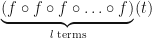
. That is, we define f_{l}(t) to be the function obtained by iterating the base function f(t)=f_{1}(t) l-1 times. One approach is to make recursive use of the Faa di Bruno formula,

\displaystyle \frac{d^{n}}{dx^{n}}f(g(x))\;=\;\sum_{k=1}^{n}f^{(k)}(g(x))B_{n,k}\left (g'(x), g''(x), \ldots, g^{(n-k+1)}(x) \right )      Eq.(1)

The fact that the exponential partial Bell polynomials B_{n,k}\left (x_{1}, x_{2},\ldots, x_{n-k+1} \right ) 
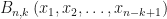
are available within the {\tt sympy} symbolic algebra Python package, makes this initially an attractive route to evaluating the required derivatives. In particular, I am interested in evaluating the derivatives at t=0 and I am focusing on odd functions of t, for which t=0 is then obviously a fixed-point. This means I only have to supply numerical values for the derivatives of my base function f(t) evaluated at t=0, rather than supplying a function that evaluates derivatives of f(t) at any point t.

Given the Taylor expansion of f(t) about t=0 we can easily write code to implement the Faa di Bruno formula using sympy. A simple bit of pseudo-code to represent an implementation might look like,

  1. Generate symbols.
  2. Generate and store partial Bell polynomials up to known required order using the symbols from step 1.
  3. Initialize coefficients of Taylor expansion of the base function.
  4. Substitute numerical values of derivatives from previous iteration into symbolic representation of polynomial.
  5. Sum required terms to get numerical values of all derivatives of current iteration.
  6. Repeat steps 4 & 5.

I show python code snippets below implementing the idea. First we generate and cache the Bell polynomials,

 # generate and cache Bell polynomials
 bellPolynomials = {}
 for n in range(1, nMax+1):
      for k in range(1, n+1):
         bp_tmp = sympy.bell(n, k, symbols_tmp)
         bellPolynomials[str(n) + '_' + str(k)] = bp_tmp

Then we iterate over the levels of function composition, substituting the numerical values of the derivatives of the base function into the Bell polynomials,

for iteration in range(nIterations):
    if( verbose ):
        print( "Evaluating derivatives for function iteration " + str(iteration+1) )

    for n in range(1, nMax+1):
        sum_tmp = 0.0
        for k in range(1, n+1):
            # retrieve kth derivative of base function at previous iteration
            f_k_tmp = derivatives_atFixedPoint_tmp[0, k-1]

            #evaluate arguments of Bell polynomials
            bellPolynomials_key = str( n ) + '_' + str( k )
            bp_tmp = bellPolynomials[bellPolynomials_key]
            replacements = [( symbols_tmp[i],
            derivatives_atFixedPoint_tmp[iteration, i] ) for i in range(n-k+1) ]
            sum_tmp = sum_tmp + ( f_k_tmp * bp_tmp.subs(replacements) )

        derivatives_atFixedPoint_tmp[iteration+1, n-1] = sum_tmp

Okay – this isn’t really making use true recursion, merely looping, but the principle is the same. The problem one encounters is that the manipulation of the symbolic representation of the polynomials is slow, and run-times slow significantly for n > 15.

However, the n^{th} derivative can alternatively be expressed as a sum over partitions of n as,

\displaystyle \frac{d^{n}}{dx^{n}}f(g(x))\;=\;\sum \frac{n!}{m_{1}!m_{2}!\ldots m_{n}!} f^{(m_{1}+m_{2}+\ldots+m_{n})}\left ( g(x)\right )\prod_{j=1}^{n}\left ( \frac{g^{(j)}(x)}{j!}\right )^{m_{j}}   Eq.(2)

where the sum is taken over all non-negative integers tuples m_{1}, m_{2},\ldots, m_{n} that satisfy 1\cdot m_{1}+ 2\cdot m_{2}+\ldots+ n\cdot m_{n}\;=\; n. That is, the sum is taken over all partitions of  n. Fairly obviously the Faa di Bruno formula is just a re-arrangement of the above equation, made by collecting terms involving f^{(k)}(g(x)) together, and as such that rearrangement gives the fundamental definition of the partial Bell polynomial.

I’d shied away from the more fundamental form of Eq.(2) in favour of Eq.(1) as I believed the fact that a number of terms had already been collected together in the form of the Bell polynomial would make any implementation that used them quicker. However, the advantage of the form in Eq.(2) is that the summation can be entirely numeric, provided an efficient generator of partitions of n is available to us. Fortunately, sympy also contains a method for iterating over partitions. Below are code snippets that implement the evaluation of f_{l}^{(n)}(0) using Eq.(2). First we generate and store the partitions,

# store partitions
pStore = {}
for k in range( n ):
    # get partition iterator
    pIterator = partitions(k+1)
    pStore[k] = [p.copy() for p in pIterator]

After initializing arrays to hold the derivatives of the current function iteration we then loop over each iteration, retrieving each partition and evaluating the product in the summand of Eq.(2). Obviously, it is relatively easy working on the log scale, as shown in the code snippet below,

# loop over function iterations
for iteration in range( nIterations ):

    if( verbose==True ):
        print( "Evaluating derivatives for function iteration " + str(iteration+1)  )

    for k in range( n ):
        faaSumLog = float( '-Inf' )
        faaSumSign = 1

        # get partitions
        partitionsK = pStore[k]
        for pidx in range( len(partitionsK) ):
            p = partitionsK[pidx]
            sumTmp = 0.0
            sumMultiplicty = 0
            parityTmp = 1
            for i in p.keys():
                value = float(i)
                multiplicity = float( p[i] )
                sumMultiplicty += p[i]
                sumTmp += multiplicity * currentDerivativesLog[i-1]
                sumTmp -= gammaln( multiplicity + 1.0 )
                sumTmp -= multiplicity * gammaln( value + 1.0 )
                parityTmp *= np.power( currentDerivativesSign[i-1], multiplicity )	

            sumTmp += baseDerivativesLog[sumMultiplicty-1]
            parityTmp *= baseDerivativesSign[sumMultiplicty-1]

            # now update faaSum on log scale
            if( sumTmp > float( '-Inf' ) ):
                if( faaSumLog > float( '-Inf' ) ):
                    diffLog = sumTmp - faaSumLog
                    if( np.abs(diffLog) = 0.0 ):
                            faaSumLog = sumTmp
                            faaSumLog += np.log( 1.0 + (float(parityTmp*faaSumSign) * np.exp( -diffLog )) )
                            faaSumSign = parityTmp
                        else:
                            faaSumLog += np.log( 1.0 + (float(parityTmp*faaSumSign) * np.exp( diffLog )) )
                    else:
                        if( diffLog > thresholdForExp ):
                            faaSumLog = sumTmp
                            faaSumSign = parityTmp
                else:
                    faaSumLog = sumTmp
                    faaSumSign = parityTmp

        nextDerivativesLog[k] = faaSumLog + gammaln( float(k+2) )
        nextDerivativesSign[k] = faaSumSign

Now let’s run both implementations, evaluating up to the 15th derivative for 4 function iterations. Here my base function is f(t) =1 -\frac{2}{\pi}\arccos t. A plot of the base function is shown below in Figure 1.

FaaDiBrunoExample_BaseFunction
Figure 1: Plot of the base function f(t)\;=\;1\;-\;\frac{2}{\pi}\arccos(t)

The base function has a relatively straight forward Taylor expansion about t=0,

\displaystyle f(t)\;=\;\frac{2}{\pi}\sum_{k=0}^{\infty}\frac{\binom{2k}{k}t^{2k+1}}{4^{k}\left ( 2k+1 \right )}\;\;\;,\;\;\;|t| \leq 1 \;\;,    Eq.(3)

and so supplying the derivatives, f^{(k)}(0), of the base function is easy. The screenshot below shows a comparison of f_{l}^{(15)}(0) for l\in \{2, 3, 4, 5\}. As you can see we obtain identical output whether we use sympy’s Bell polynomials or sympy’s partition iterator.
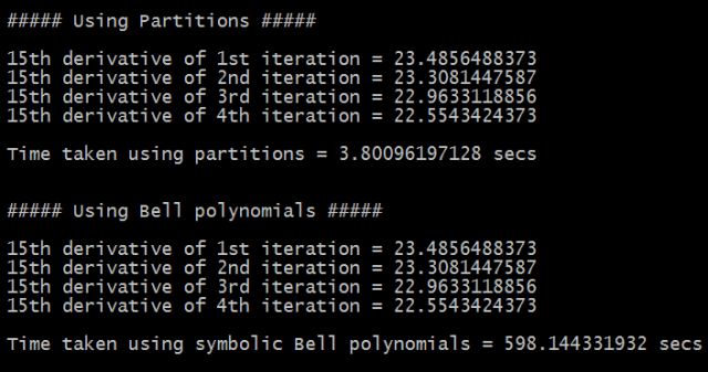
FaaDiBruno_TimingComparison

The comparison of the implementations is not really a fair one. One implementation is generating a lot of symbolic representations that aren’t really needed, whilst the other is keeping to entirely numeric operations. However, it did highlight several points to me,

  • Directly working with partitions, even up to moderate values of n, e.g. n=50, can be tractable using the sympy package in python.
  • Sometimes the implementation of the more concisely expressed representation (in this case in terms of Bell polynomials) can lead to an implementation with significantly longer run-times, even if the more concise representation can be implemented concisely (less lines of code).
  • The history of the Faa di Bruno formula, and the various associated polynomials and equivalent formalisms (such as the Jabotinksy matrix formalism) is a fascinating one.

I’ve put the code for both methods of evaluating the derivatives of an iterated function as a gist on github.

At the moment the functions take an array of Taylor expansion coefficients, i.e. they assume the point at which derivatives are requested is a fixed point of the base function. At some point I will add methods that take a user-supplied function for evaluating the k^{th} derivative, f^{(k)}(t), of the base function at any point t and will return the derivatives, f_{l}^{(k)}(t) of the iterated function.

I haven’t yet explored whether, for reasonable values of n (say n \leq 50), I need to work on the log scale, or whether direct evaluation of the summand will be sufficiently accurate and not result in overflow error.

Manchester R User Group Meetup – May 2017

At the latest Manchester R User Group meeting (organized by Mango Solutions) Leanne Fitzpatrick from HelloSoda gave a talk on Deploying Models in a Machine Learning Environment.

Leanne spoke about how the use of Docker had speeded up the deployment of machine learning models into the production environment, and had also enabled easier monitoring and updating of the models.

One of the additional benefits, and Leanne alluded that this may even have been the original motivation, was that of reducing the barriers between the data scientists and software engineers in the company. Data Science is an extremely broad church, encompassing a wide range of skill-sets and disciplines. Inevitably, there can be culture-clashes between those who consider themselves to be from the ‘science’ side of Data Science, and those from the engineering side of Data Science. Scientists are people who like to explore data, develop proof-of-concept projects, but who are often not the most disciplined in code writing and organization, and for whom operational deployment of a model is the last stage in their thinking. Scientists break things. Scientists like to break things. Scientists learn by breaking things.

xkcd_the_difference
Scientists are different (taken from xkcd.com)

Data Scientists who break things can be seen as an annoyance to those responsible for maintaining the operational infrastructure.

Obviously, in a commercial environment the data scientists and software engineers/developers need to work as efficiently together as possible. The conclusion that Leanne presented in her talk suggested that HelloSoda have taken some steps towards solving this problem through their use of containerization of the models.  I say, ‘some steps’, as I can’t believe that any organization can completely remove all such barriers. Having worked in inter-disciplinary teams in both the commercial world and in academic research I’ve seen some teams work well together and others not. What tools and protocols an organization can use to generally reduce the barriers between investigative Data Science and operational Data Science is something that intrigues me – something for a longer post maybe.

SciPy incomplete gamma function

I got tripped up by this recently when doing eigenvalue calculations in python. I wanted to evaluate the incomplete gamma function \gamma (a, x)\;=\;\int_{0}^{x}t^{a-1}e^{-t}dt. After using the SciPy {\tt gammainc} function I was scratching my head as to why I was seeing a discrepancy between my numerical calculations for the eigenvalues and my theoretical calculation. Then I came across this post by John D Cook that helped clarify things. The SciPy function {\tt gammainc} actually calculates \gamma(a,x)/\Gamma(a).